Diffusion Models – More Than Adding Noise
Dr J Rogel-Salazar2022-10-04 | 12 min read
Go to your favourite social media outlet and use the search functionality to look for DALL-E. You can take a look at this link to see some examples in Twitter. Scroll a bit up and down, and you will see some images that, at first sight, may be very recognisable. Depending on the scenes depicted, if you pay a bit more attention you may see that in some cases something is not quite right with the images. At best there may be a bit (or a lot) of distortion, and in some other cases the scene is totally wacky. No, the artist did not intend to include that distortion or wackiness, and for that matter it is quite likely the artist is not even human. After all, DALL-E is a computer model, called so as a portmanteau of the beloved Pixar robot Wall-E and the surrealist artist Salvador Dalí.
The images you are seeing have been generated digitally from text input. In other words, you provide a description of the scene you are interested in, and the machine learning model creates the image. What a future we are living in, right? The DALL-E model was announced in January 2021 by OpenAI, and more recently DALL-E 2 entered into a beta phase in late July 2022. In late August 2022 OpenAI introduced Outpainting – a way to continue an image beyond its original borders. Different implementations have since been released and you can play with a variety that are out there. For example, take a look at Craiyon to get your very own AI image creations from text.
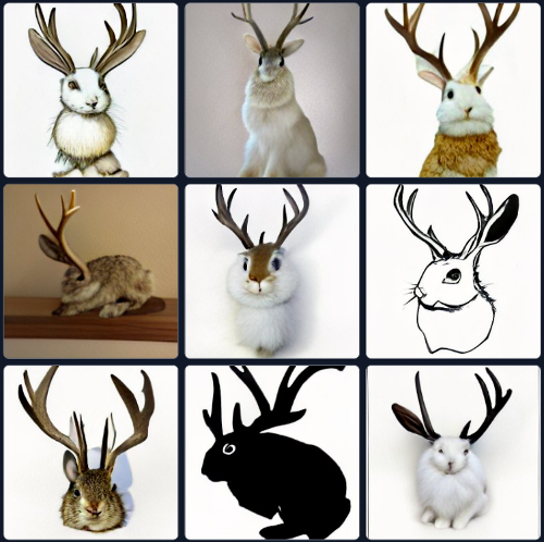
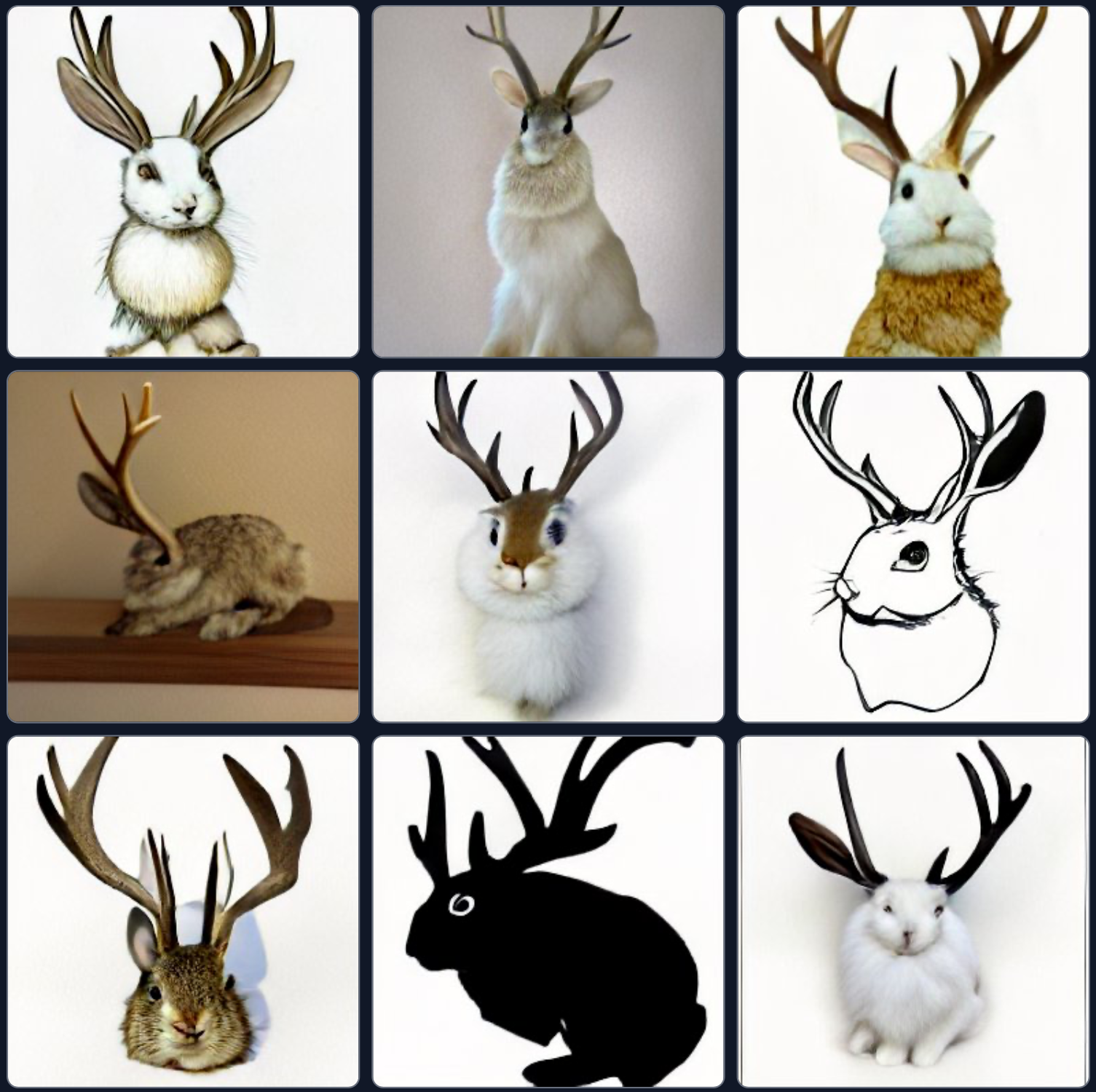
Below are some example for a request I did to get images of jackalopes - you may know I refer to them as an allegory of a data scientist… for more information take a look at Data Science and Analytics with Python. In any case, you can see that some of the depictions obtained are rather good for example the third entry on the second row shows a plausible drawing of what is clearly a hare with deer-like antlers. In other cases the result is not that great, look for instance at the second entries of rows 1 and 2 – the heads are decidedly the wrong size for the bodies chosen, too small in one case, and too big in the other one. In any event, I would not have been as fast at creating these many examples in the short time it took Craiyon (formerly known as DALL-E mini) to create them.
The original DALL-E implementation released by OpenAI uses a version of GPT-3, if you need to learn more about that check my post in this site entitled “Transformers - Self-attention to the rescue”. Together with Contrastive Language-Image Pre-training, or CLIP for short, and diffusion modelling, DALL-E is able to generate images in multiple styles and arrangements. The focus of this blog post is on exploring what is behind diffusion models. Let us get started.
What Are Diffusion Models?
Like many great concept extensions, inspiration for diffusion models comes from physics, and in this case the name used is not shy to show its roots. Diffusion is a process where something - atoms, molecules, energy, pixels - move from a region of higher concentration to another one of lower concentration. You are familiar with this when you dissolve sugar in a cup of coffee. At first the sugar granules are concentrated at the top of your mug in a specific place, and if left on their own they will randomly move around and distribute themselves. If you aid the process by stirring, the concentration gradient is accelerated and you can enjoy your sweetened coffee keeping you awake while reading these lines.
As we mentioned above, a diffusion model in machine learning takes inspiration from diffusion in non-equilibrium thermodynamics, where the process increases the entropy of the system. This means that the diffusion process is spontaneous and irreversible, in other words, particles (atoms, pixels, etc.) spread out by the process but will not spontaneously re-order themselves. In terms of information theory, this is equivalent to losing information due to the extra noise added.
In the paper titled “Deep Unsupervised Learning using Non-Equilibrium Thermodynamics” by Sohl-Dickstein et al. the motivation provided by non-equilibrium statistical physics is at the centre of their approach. The idea is to exploit the effects of diffusion by slowly perturbing and destroying the structure of the data distribution at hand. Unlike the physical process, the aim is to learn a reverse diffusion (shall that be called concentration?) process to restore and generate structure in the data.
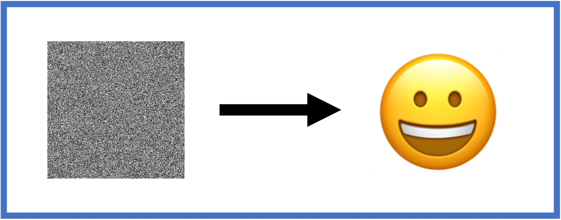
Like in a thermodynamic approach, we define a Markov chain of diffusion steps to add systematically random noise to our data. The learning of the reverse diffusion process enables us to construct data samples from the noise with the desired properties, in this case, like in the image below going from a noisy image to a smiley face emoji.
In a nutshell we are talking about a two-step process:
- A forward diffusion step where Gaussian noise is added systematically until the data is actually noise; and
- A reconstruction step where we “denoise” the data by learning the conditional probability densities using neural networks.
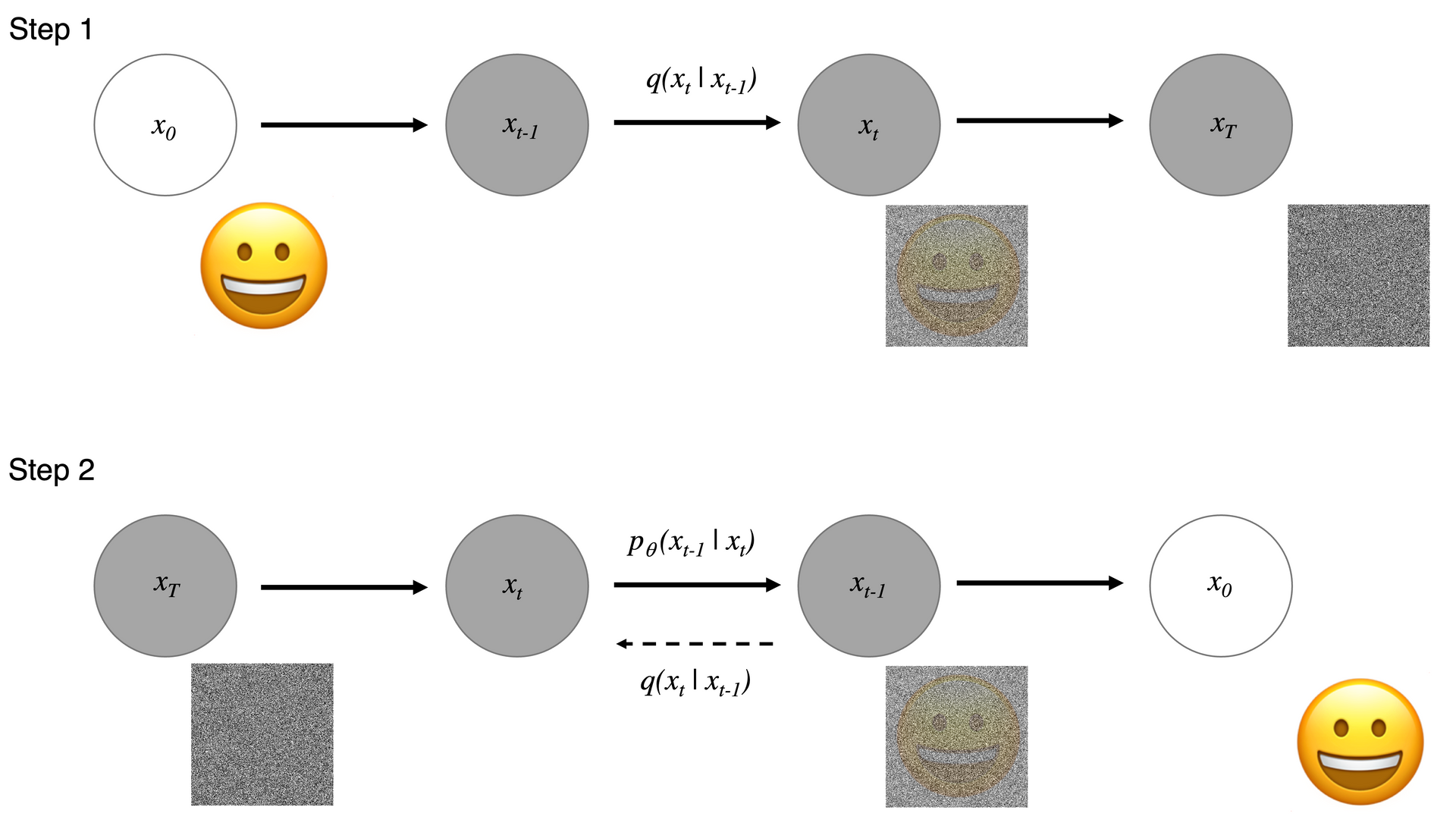
Consider the diagram above for the two steps we have outlined. For a data point from a real data distribution \(x_0 \simeq q(x) \), the forward diffusion process adds small Gaussian noise to the sample in $T$ Steps. The step sizes are controlled by a variance schedule such that \( \{\beta_t \in (0,1) \}^T_{t=1} \), and we have that \( q(x_t | x_{t-1} = N (x_t; \sqrt{1-\beta_t} x_{t-2}, \beta_t I) \). In our diagram, for Step 1 we start with a smiley face emoji at \( x_0 \). As we add noise at each step, we wash away the original image. At the point when \( T \to \infty \), we have an isotropic Gaussian distribution.
During our second step, we take a noisy image and we are interested in reconstructing our smiley face emoji. This works under the assumption that if we can reverse the process in Step 1, we can recreate the true sample from Gaussian noise input. Sadly, we can’t easily estimate \( q(x_{t-1} | x_t) \) , and hence the need to learn a model \( p_{\theta} \) to reverse the diffusion process. This is where the magic of image generation happens. The Markov formulation in which the model is based ensures that a given reverse diffusion transition distribution only depends on the previous time step allowing us to evolve the process.
When training our diffusion model, we are in effect finding the reverse Markov transitions that maximise the likelihood of the training data.
Image Generation with Different Methodologies
If generating an image is the name of the game, there may be other alternatives to the diffusion models described above. Let us look at some options and compare and contrast them to diffusion models.
One possibility for our image generation is the use of Variational Autoencoders (VAEs) which take an input that is encoded by reducing it to a latent space of lower dimensionality. When we decode the result, the model is trying to reconstruct the input, hence generating our image. Note that VAEs not only are asked to generate our images, but also to represent them in a more compact way (dimensionality reduction). This means that the model is effectively learning the essential features of the probability distribution that generated the training data. This may be a disadvantage in some cases.
Another possibility usually mentioned in this context is the use of flow-based models. In this case, we do not use encoders and decoders. Instead, we use a sequence of invertible transformations to directly model a probability distribution. Instead of encoding the input, we use a function \( f \) parametrised by a neural net unto our data. When retrieving the result, we simply use the inverse of our function, i.e. \( f^{-1} \). We can see how this can become an issue.
A third possibility is the use of GANs. A Generative Adversarial Network (GAN) is an approach to generative modelling using deep learning. In effect, it consists in learning patterns in input data such that the model can be employed to generate new examples that can plausibly have been drawn from the original data. In a GAN architecture we have a couple of neural nets what are competing with one another to generate synthesised instanced of the data. In a previous post in this blog we have talked about the advantages of using GANs . To generate images from noise with a GAN our starting point is noise of a useful conditioning variable. Images are generated by the so-called generator, and the results are judged by the discriminator to be (or not) good plausible data drawn from the training set. Some areas that require our attention when using GANs are: the potential for vanishing gradients in cases where the discriminator is too good; or model collapse in cases where the generator learns to produce only specific output, cornering the discriminator into rejecting anything and everything. In a paper published in 2021 Diffusion Models Beat GANs on Image Synthesis, Dhariwal et al. show how “diffusion models can achieve image sample quality superior to the current state-of-the-art generative models.”
Diffusion models seem to be getting the upper hand at generating images, however, they are not without issues. In a recent two-part article (Part 1 and Part 2), researchers at NVIDIA have argued that although diffusion models achieve high sample quality and diversity, they are not great in sampling speed limiting their adoption in practical every-day applications. They then go on to present three techniques developed at NVIDA to address this issue, namely:
- Latent space diffusion models to simplify the data by first embedding it into a smooth latent space, where a more efficient diffusion model can be trained.
- Critically damped Langevin diffusion, an improved forward diffusion process well suited for easier and faster denoising and generation.
- Denoising diffusion GANs directly learn a significantly accelerated reverse denoising process through expressive multimodal denoising distributions.
Diffusion modelling has been shown to be a very robust approach in image generation. What is more, advances in the production of audio and video based on the same approach have been demonstrated. Next time you are looking at a noisy image or listen to some something that sounds quite literally like noise to you, stop to consider that it may be the beginning of a beautiful scene, a moving film, or a fantastic symphony. Who would have thought!
Dr Jesus Rogel-Salazar is a Research Associate in the Photonics Group in the Department of Physics at Imperial College London. He obtained his PhD in quantum atom optics at Imperial College in the group of Professor Geoff New and in collaboration with the Bose-Einstein Condensation Group in Oxford with Professor Keith Burnett. After completion of his doctorate in 2003, he took a posdoc in the Centre for Cold Matter at Imperial and moved on to the Department of Mathematics in the Applied Analysis and Computation Group with Professor Jeff Cash.
RELATED TAGS
SHARE
Subscribe to the Domino Newsletter
Receive data science tips and tutorials from leading Data Science leaders, right to your inbox.
By submitting this form you agree to receive communications from Domino related to products and services in accordance with Domino's privacy policy and may opt-out at anytime.