Feature extraction and image classification using Deep Neural Networks and OpenCV

In a previous blog post we talked about the foundations of Computer vision, the history and capabilities of the OpenCV framework, and how to make your first steps in accessing and visualising images with Python and OpenCV. Here we dive deeper into using OpenCV and DNNs for feature extraction and image classification.

Image classification and object detection

Image classification is one of the most promising applications of machine learning aiming to deliver algorithms with the capability to recognise and classify the content of an image with a near human accuracy.

The image classification approaches are typically divided into traditional methods, based on extraction of images features and their utility in classification, or more advanced approaches that exploit the strength of deep neural networks.

Traditional approaches with feature extraction

There are various features that can potentially be extracted using different machine learning algorithms. Lowe et al. (2004) developed Scale Invariant Feature Transform (SIFT) aiming to solve intensity, viewpoint changes and image rotation in feature matching [1]. SIFT allows estimation of scale-space extrema followed by keypoint localisation, orientation and subsequently computation of local image descriptor for each key point. Moreover, SIFT offers efficient recognition of objects in a given image, however, its implementation is computationally expensive and time-consuming.

SIFT has inspired the development of other variants in particular to overcome the complexity and the associated computational demand. One such variant is Speed up Robust Feature (SURF), which reportedly outperforms SIFT without a negative impact on the robustness of detected points and overall model accuracy [2]. Another alternative to SIFT is Robust Independent Elementary Features (BRIEF) offering similar performance with significantly less complexity [3]. Furthermore, Rublee et al., (2011) reported that Oriented FAST and Rotated BRIEF (ORB) provides more efficient performance [4].

Additionally, Histogram of Oriented Gradients (HOG) HOG is utilised in various tasks including object detection allowing the occurrence of edge orientations to be measured. In principle, this descriptor is representative of a local statistic of the orientations for the image gradients for a key point. Simply, each descriptor can be considered as a collection of histograms that are composed of pixel orientations assigned by their gradients [5].

SIFT

Scale-Invariant Feature transform was initially proposed by David Lowe in 2004 as a method for extracting distinctive invariant features from images with the view to use it for feature matching between images. This is a particularly useful approach as it can detect image features irrespective of orientation and size [1]. Below we provide the steps required to extract SIFT from the "face" image displayed in the previous step (see the "Opening and displaying the image file" section in the previous blog post).

sift = cv2.xfeatures2d.SIFT_create()
original_keypoints, original_descriptor = sift.detectAndCompute(gray_face, None)
query_keypoints, query_descriptor = sift.detectAndCompute(query_face_gray, None)
keypoints_without_size = np.copy(original_face)
keypoints_with_size = np.copy(original_face)

cv2.drawKeypoints(original_face, original_keypoints, keypoints_without_size, color = (0, 255, 0))
cv2.drawKeypoints(original_face, original_keypoints, keypoints_with_size, flags = 
cv2.DRAW_MATCHES_FLAGS_DRAW_RICH_KEYPOINTS)

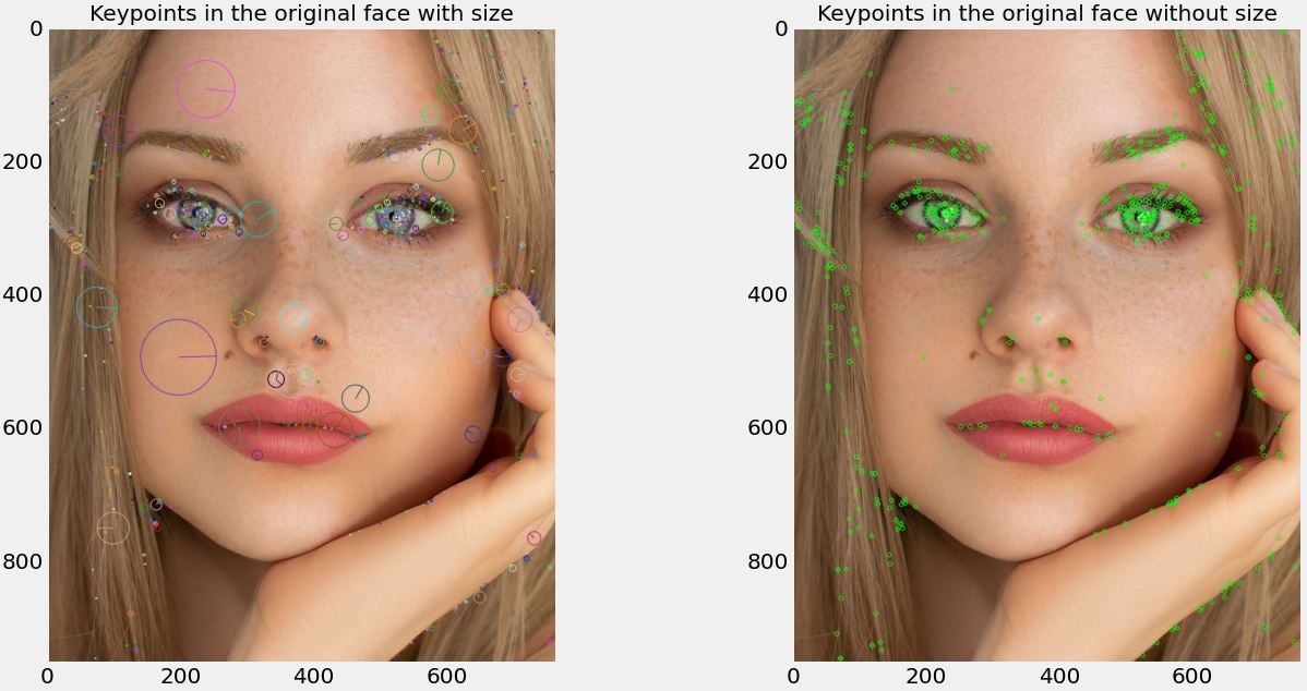
Figure 1. Keypoints detected with/without size in the left and right images respectively

FAST

Features from accelerated segment test (FAST) is a corner detection method to extract feature points originally proposed by Edward Rosten and Tom Drummond in 2006. This method is very efficient and thus suitable for resource-intensive applications including real-time video processing [6]. Below we will provide the steps required to extract SIFT from the "face" image displayed in the previous step.

fast = cv2.FastFeatureDetector_create() 
keypoints_with_nonmax = fast.detect(gray_face, None)
fast.setNonmaxSuppression(False)
keypoints_without_nonmax = fast.detect(gray_face, None)
image_with_nonmax = np.copy(original_face)
image_without_nonmax = np.copy(original_face)
cv2.drawKeypoints(original_face, keypoints_with_nonmax, image_with_nonmax, color=(0,255,0),
flags=cv2.DRAW_MATCHES_FLAGS_DRAW_RICH_KEYPOINTS)
cv2.drawKeypoints(original_face, keypoints_without_nonmax, image_without_nonmax, color=(0,255,0), 
flags=cv2.DRAW_MATCHES_FLAGS_DRAW_RICH_KEYPOINTS)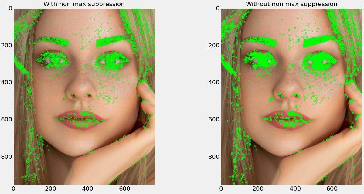

Figure 2. Keypoints detected with/without non-max suppression.

ORB

Oriented FAST and Rotated BRIEF (ORB) was originally proposed by Ethan Rublee, Vincent Rabaud, Kurt Konolige, and Gary R. Bradski in 2011 (OpenCV Labs). This method is rotation invariant and resistant to noise. The main rationale was to provide a more efficient alternative to SIFT and SURF that is free to use without any restriction [4]. SIFT and SURF are, however, still patented algorithms. We will use the same image for the extraction of ORB descriptors.

orb = cv2.ORB_create()
original_keypoints, original_descriptor = orb.detectAndCompute(gray_face, None)
query_keypoints, query_descriptor = orb.detectAndCompute(query_face_gray, None)
keypoints_without_size = np.copy(original_face)
keypoints_with_size = np.copy(original_face)

cv2.drawKeypoints(original_face, original_keypoints, keypoints_without_size, color = (0, 255, 0))
cv2.drawKeypoints(original_face, original_keypoints, keypoints_with_size, flags = 
cv2.DRAW_MATCHES_FLAGS_DRAW_RICH_KEYPOINTS)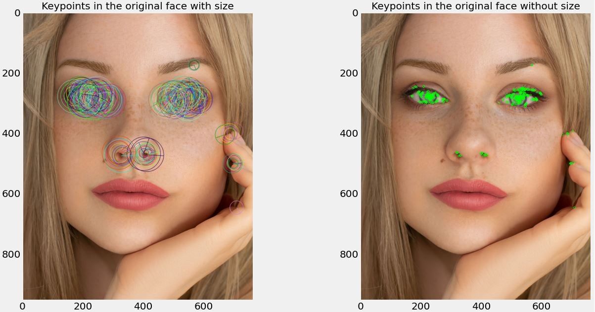

Figure 3. Keypoints detected with/without size in the left and right images respectively.

brute_force = cv2.BFMatcher(cv2.NORM_HAMMING, crossCheck = True)
matches = brute_force.match(original_descriptor, query_descriptor)
matches = sorted(matches, key = lambda x : x.distance)
result = cv2.drawMatches(original_face, original_keypoints, query_face_gray, query_keypoints, matches, 
query_face_gray, flags = 2)
print("The number of matching keypoints between the original and the query image is {}\n".format(len(matches)))

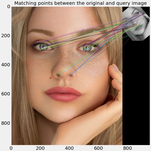
Figure 4. Matching of keypoints detected in the original (main) and query (top) images.

Classification using OpenCV DNN and pre-trained DenseNet

OpenCV can be utilised to solve image classification problems. The OpenCV library offers a Deep Neural Network (DNN) module, which facilitates the use of deep learning related functions within OpenCV. This module was introduced in OpenCV version 3 and this tutorial is using OpenCV v4.5.2. The main function of the DNN module is that it allows transfer learning and the use of pre-trained models. Note that the DNN modules cannot be used to train models but work with models that are trained using other popular neural network frameworks including PyTorch, TensorFlow, Caffe, Darknet and ONNX.

There are several advantages of using OpenCV DNN for inference only. Offloading model training to other libraries and using pre-trained models leads to simple and straightforward code. This makes it easier to adopt CV concepts and onboard users who don't necessarily have deep understanding of DNNs. Furthermore, this approach offers support to OpenCL-based Intel GPUs in addition to CUDA-based NVIDIA CPUs allowing for higher performance.

In this tutorial, we will use the pre-trained DenseNet121 model, trained using the Caffe framework on the ImageNet database, which consists of 1000 image classes. A DenseNet is a type of convolutional neural network (CNN) that uses dense connections between layers (via Dense Blocks). All layers with matching feature-map sizes are connected directly with each other. To use the pre-trained DenseNet model we will use the OpenCV for loading the model architecture and pre-trained weights. In this process we will perform the following steps:

1. Image pre-processing
2. Loading class labels
3. Initialising the model
4. Classification and visualising the output

The images were obtained from Unsplash, which offers free stock images. The images offered can be used for commercial and non-commercial purposes and no permission for use is required. Prior to feeding the image into the model, some pre-processing is required. These include resizing the images to 224x224, as required by the model, setting scale, and cropping the images where necessary. The pre-processing is handled by the OpenCV's cv2.dnn.blobFromImage() function.

Next, we load the ImageNet image classes, create a labels list, and initialise the DNN module. OpenCV is capable to initialise Caffe models using cv2.dnn.readNetFromCaffe, TensorFlow models using cv2.dnn.readNetFromTensorFlow, and PyTorch models using cv2.dnn.readNetFromTorch, respectively. This choice is determined by the original framework that the model was trained under. DenseNet121 was trained using Caffe and thus we will initialise the DNN module using cv2.dnn.readNetFromCaffe. The pre-processed image is fed to the network and undergoes a series of computations in the forward pass phase.

def image_classification(model_weights, model_architecture, image):   
    blob = cv2.dnn.blobFromImage(image, 0.017, (224, 224), (103.94,116.78,123.68))
    global model, classes
    rows = open('Resources/model/denseNet/synset_words.txt').read().strip().split("\n")
    image_classes = [r[r.find(" ") + 1:].split(",")[0] for r in rows]
    model = cv2.dnn.readNetFromCaffe(model_architecture, model_weights)  
    model.setInput(blob)    
    output = model.forward()    
    new_output = output.reshape(len(output[0][:]))   
    expanded = np.exp(new_output - np.max(new_output))
    prob =  expanded / expanded.sum()    
    conf= np.max(prob)    
    index = np.argmax(prob)
    label = image_classes[index]   
    text = "Label: {}, {:.2f}%".format(label, conf*100)
    cv2.putText(image, "{}: {:.2f}% confidence".format(label, conf *100), (5, 40), cv2.FONT_HERSHEY_COMPLEX, 1, (255, 255, 255), 2)
model_architecture ='Resources/model/denseNet/DenseNet_121.prototxt.txt'
model_weights = 'Resources/model/denseNet/DenseNet_121.caffemodel'
image1 = cv2.imread('Resources/images/persian_cat.jpg')
classify1 = image_classification(model_weights, model_architecture, image1)
image2 = cv2.imread('Resources/images/dog.jpg')
classify2 = image_classification(model_weights, model_architecture, image2)

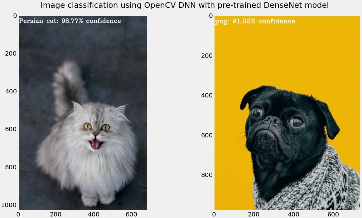
Figure 5. Image classification using OpenCV DNN module with pre-trained DenseNet model. For the images used in this figure, both classified names were correct with 98.7 and 91% for Persian cat and Pug classification, respectively.

Object detection

For object detection, we will use two approaches: Haar cascades and OpenCV DNN module together with MobileNet SSD pre-trained model.

Haar cascades, introduced by Viola and Jones in 2001 [7] is an approach that can detect objects in images irrespective of the scale and location of those objects in the image. The authors were primarily concerned with face detection, although their method can be adapted to allow detection of other objects. This is a fast method compared to more advanced approaches, but consequently the accuracy of the Haar cascade is lower. In many cases it produces a large number of false positives.

OpenCV DNN module with MobileNet SSD pre-trained model. This method receives pre-processed images and feeds them to a pre-trained model. We will show it in action and then visualise the output for two different images. We will use MobileNet Single Shot Detector (SSD) trained originally on the COCO dataset using the TensorFlow deep learning framework. SSD models typically offer higher performance in terms of computation time compared to other alternatives and thus are more suitable for this tutorial.

Object detection using Haar Cascade

To illustrate the use of Haar cascades we'll show how to detect eyes and faces in humans and faces in cats. The implementation is as follows.

face_cascade = cv2.CascadeClassifier("Resources/model/haarcascades/haarcascade_frontalface_default.xml")
eye_cascade = cv2.CascadeClassifier("Resources/model/haarcascades/haarcascade_eye.xml")

img = cv2.imread("Resources/images/group.jpg")
gray = cv2.cvtColor(img, cv2.COLOR_BGR2GRAY)
faces = face_cascade.detectMultiScale(gray, 1.3, 5)

for (x,y,w,h) in faces:
    img1 = cv2.rectangle(img,(x, y),(x + w, y + h),(255,255,0),2)
    roi_gray = gray[y: y + h, x: x + w]
    roi_color = img[y: y + h, x: x + w]
    eyes = eye_cascade.detectMultiScale(roi_gray)
    for (ex, ey, ew, eh) in eyes:
        cv2.rectangle(roi_color,(ex, ey), (ex + ew, ey + eh), (0,255,0),2)
 
cat_face_cascade = cv2.CascadeClassifier("Resources/model/haarcascades/haarcascade_frontalcatface.xml")
img = cv2.imread("Resources/images/cats.jpg")
img_rgb = cv2.cvtColor(img, cv2.COLOR_BGR2RGB)
faces = cat_face_cascade.detectMultiScale(img_rgb, 1.1, 4)

for (x,y,w,h) in faces:
    img2 = cv2.rectangle(img_rgb,(x, y),(x + w, y + h),(255,255,0),5)

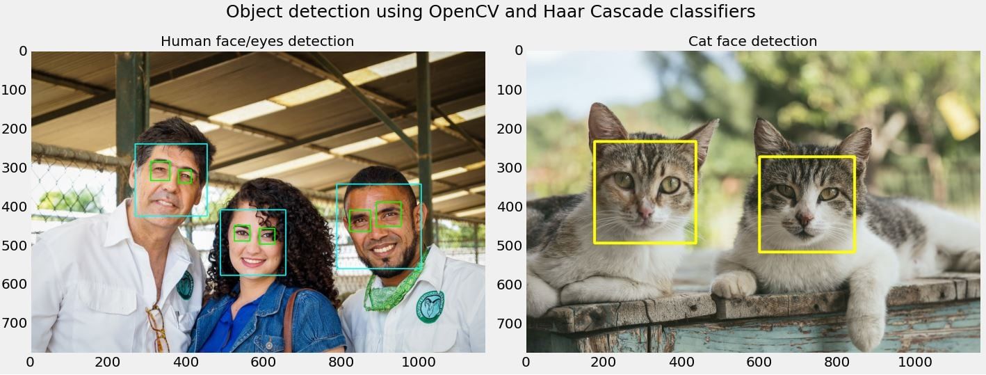
Figure 6. Object detection using Haar cascade classifiers. The image on the left is the result of eye and face detection for humans and the image on the right is the output for cat face detection.

Object detection using OpenCV DNN and pre-trained MobileNet

We aim to detect objects in two images depicted in Figure 7 using the following code.

def detect_objects(model_architecture, config, framework, image):
    image_height, image_width, _ = image.shape
    blob = cv2.dnn.blobFromImage(image, size=(300, 300), mean=(104, 117, 123), swapRB=True)
    global model, classes    
    with open('Resources/model/mobileNet/object_detection_classes_coco.txt', 'r') as f:
        class_names = f.read().split('\n')    
    model = cv2.dnn.readNet(model_architecture, config, framework)
    model.setInput(blob)   
    output = model.forward()
    colours = np.random.uniform(0, 255, size=(len(class_names), 3))
    for detection in output[0, 0, :, :]:
       confidence = detection[2]
       if confidence > .4:
           class_id = detection[1]
           class_name = class_names[int(class_id)-1]
           color = colours[int(class_id)]
           box_x = detection[3] * image_width
           box_y = detection[4] * image_height
           box_width = detection[5] * image_width
           box_height = detection[6] * image_height
           cv2.rectangle(image, (int(box_x), int(box_y)), (int(box_width), int(box_height)), color, 2)
           cv2.putText(image, class_name, (int(box_x), int(box_y - 5)), cv2.FONT_HERSHEY_SIMPLEX, 1, color, 2)

model_architecture = 'Resources/model/mobileNet/frozen_inference_graph.pb'
config = 'Resources/model/mobileNet/ssd_mobilenet_v2_coco_2018_03_29.pbtxt'
framework='TensorFlow'
image1 = cv2.imread('Resources/images/dogcats.jpg')
detect1 = detect_objects(model_architecture, config, framework, image1)
image2 = cv2.imread('Resources/images/dogs_humans.jpg')
detect2 = detect_objects(model_architecture, config, framework, image2)

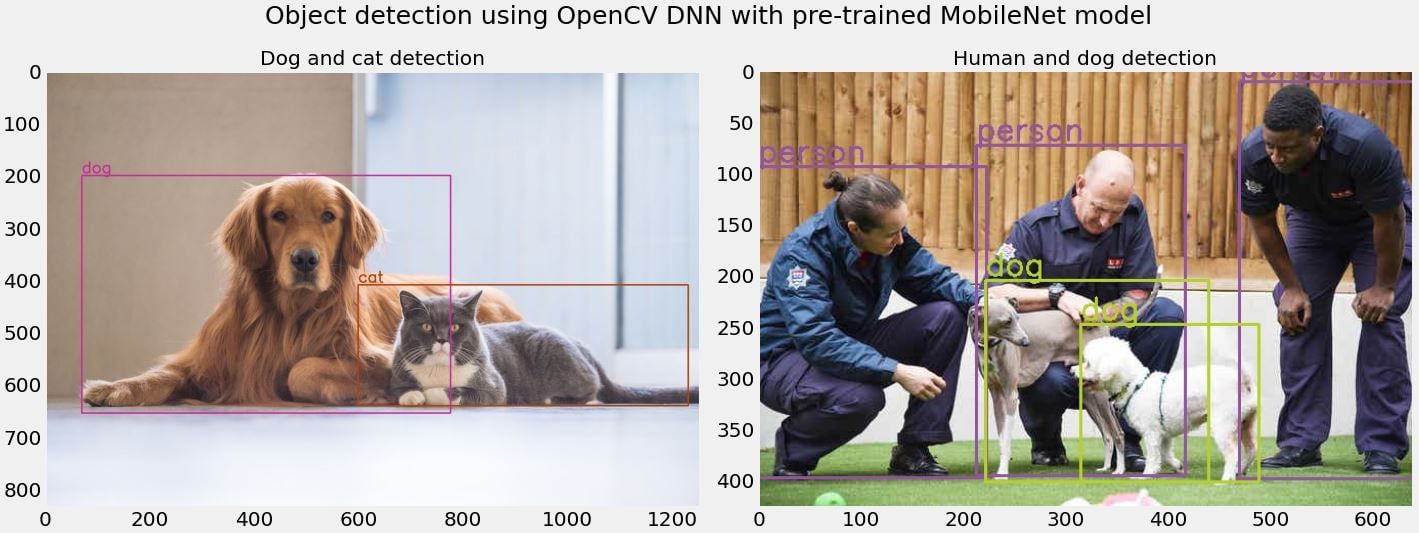
Figure 7. Object detection using OpenCV and pre-trained MobileNet. In both images were a mixture of animals on the left image and animals with humans on the right image are present, this object detection method resulted in accurate labelling of the objects with appropriate corresponding bounding boxes around the objects.

Conclusion

OpenCV is one of the main libraries utilised in computer vision. Herein, we covered a brief background on this powerful library and described the steps required for feature extraction, image classification and object detection.

The profound advancement in neural networks and deep learning over the past 10 years have resulted in significant progress in computer vision. OpenCV is one of the libraries that has made this journey possible, and we hope to have provided sufficient information to encourage our readers to seek further training on the many functions offered by OpenCV in solving their computer vision problems.

Additional Resources

You can check the following additional resources:

• Read our blog on Getting Started with OpenCV
• Free online courses on OpenCV - https://opencv.org/opencv-free-course/
• OpenCV official documentation - https://docs.opencv.org/4.x/
• There is an accompanying project with all code from this article, which you can access by signing up for the free Domino MLOps trial environment:

References

[1] D. G. Lowe, "Distinctive image features from scale-invariant keypoints," International journal of computer vision, vol. 60, no. 2, pp. 91-110, 2004.

[2] H. Bay, A. Ess, T. Tuytelaars, and L. Van Gool, "Speeded-up robust features (SURF)," Computer vision and image understanding, vol. 110, no. 3, pp. 346-359, 2008.

[3] M. Calonder, V. Lepetit, C. Strecha, and P. Fua, "Brief: Binary robust independent elementary features," in European conference on computer vision, 2010: Springer, pp. 778-792.

[4] E. Rublee, V. Rabaud, K. Konolige, and G. Bradski, "ORB: An efficient alternative to SIFT or SURF," in 2011 International conference on computer vision, 2011: Ieee, pp. 2564-2571.

[5] D. Monzo, A. Albiol, J. Sastre, and A. Albiol, "Precise eye localization using HOG descriptors," Machine Vision and Applications, vol. 22, no. 3, pp. 471-480, 2011.

[6] E. Rosten and T. Drummond, "Machine learning for high-speed corner detection," in European conference on computer vision, 2006: Springer, pp. 430-443.

[7] P. Viola and M. Jones, "Rapid object detection using a boosted cascade of simple features," in Proceedings of the 2001 IEEE computer society conference on computer vision and pattern recognition. CVPR 2001, 2001, vol. 1: Ieee, pp. I-I.