GPU-accelerated Convolutional Neural Networks with PyTorch

Convolutional Neural Networks (CNNs and also ConvNets) is a class of Neural Networks typically used for image classification (mapping image data to class values). At a high level, CNNs can be viewed simply as a variant of feedforward networks, but they have a number of advantages in comparison to more traditional algorithms for analysing visual imagery.

• CNNs leverage the hierarchical nature of visual compositions, starting with simple primitives and combining them to produce patterns of increasing complexity. This has the ultimate effect of automating the feature selection phase, which gives ConvNets an advantage against other techniques that rely on handcrafted features.
• Being neural networks, CNNs also benefit from a scalable architecture and are also suitable for GPU-accelerated training. This makes them a good option for processing large datasets.
• Classical feedforward neural networks are fully connected, which means they are computationally heavy and, with the increase of their number of parameters, are prone to overfitting. On the other hand, the convolutional and pooling layers of ConvNets reduce the original dimensionality before feeding the data to a fully connected layer, thus making the network computationally lighter and less likely to overfit.

Convolving images

At the heart of CNNs is the convolution - a process that transforms the input image (a matrix) by applying a kernel (another matrix) over each pixel of the image and its neighbours. From a mathematical standpoint, a convolution operation produces a function that shows how a second function modifies a third function. Without getting into the mathematical details, the intuition behind using convolution for image processing is as follows: the original image is taken as a matrix, where each element represents a single pixel. These can be either zeros or ones (for a monochrome image) or integers in a given range (e.g. 0-255 to denote the intensity in a grayscale image). For colour images we typically use multiple matrices, one for each channel and things get slightly more complicated but the principles are the same.

A convolutional layer in a CNNs uses a kernel or a filter, which is simply another matrix of smaller dimensions (e.g. 3x3, 5x5 etc.). The kernel is slid over the image, operating over patches of identical size. The current patch and the kernel are then convolved by performing element-wise matrix multiplication and adding the resulting elements together to produce a single scalar. This process is illustrated below.

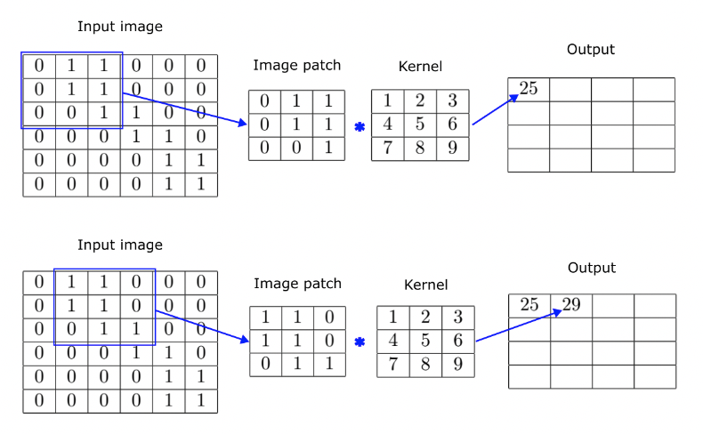
The kernel in this example is of size 3x3, so we take a 3x3 patch from the original image starting at its top left corner. The image patch and the kernel are convolved to produce a single scalar value - 25. Then we slide the selection to the right and take a second patch to produce the second output element. We repeat the operation until we exhaust all possible patches in the original image. Notice, that with a 3x3 patch we can do four slides on the horizontal and another four vertically. Therefore, the result of applying a 3x3 kernel over a 6x6 image is a 4x4 output matrix. This also demonstrates how convolution achieves dimensionality reduction, but this is typically not the main mechanism we rely on for reducing the output size.

Let's observe the effects of convolving a random image with a couple of kernels. First, we start with the original image - a photo of the beautiful Atari 800 8-bit home computer.

Convolving this image with the following kernel

results in an image that is slightly blurred.

This transformation is not easy to spot, but the results are not always that subtle. For example, we can convolve the original image with the following kernel.

This yields the following output image:

This transformation is very useful for edge detection. Also note, that in this case we have preserved the original image dimensions. The simplest way to do this is to pad the original image with zeros around the border so that we get a number of patches identical to its original resolution. We mention this only for clarity, as this is really not essential to understanding how convolving an image with a kernel works.

Now, if you take a step back and think about the output result of applying a filter you'll realise that you can look at filters as feature detectors. For example, in the image above we see how much each image patch features something that resembles an edge. You can be much more precise by using various kernels that can detect only horizontal, or only vertical edges. You could use kernels that detect arches, diagonals and so on. Sliding the image patch window over the image and using an appropriate kernel is essentially a pattern detection mechanism.

Architecture of a convolutional neural network

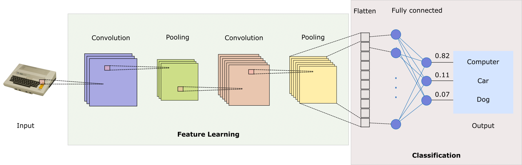
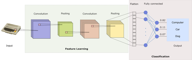
Now that we understand how convolutions are used as the building blocks of a CNN, let's talk about what the typical network architecture looks like. Generally speaking, a CNN network has two functionally distinct elements — one is responsible for the feature extraction, and the other one for performing classification based on the extracted features.

The feature extraction (or feature learning) part of the network employs a series of convolutional and pooling layers.

• Each convolutional layer applies a filter, which is convolved with the input to create an activation map. As we already showed in the previous section, the filter is slid over the image (both horizontally and vertically) and an output scalar is calculated for each spatial position. If the image contains data about colour, the typical approach is to process each colour channel separately, producing a tensor instead of a simple 2D matrix.
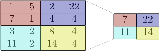
• Convolutional layers generally preserve the dimensionality of the input. This may be problematic, because the same feature (e.g. an edge or a straight line) if present in different places in the image results in different feature maps. Pooling layers is what ConvNets use to address this challenge. These layers downsample the image to lower resolutions in a way that also preserves the features present in the feature map.
  
  
  The image above shows a max pooling layer that summarises the most activated features from a 4x4 feature map. You see that the pooling layer partitions the feature map into four regions and creates a single scalar with the maximum for each patch. This is an example of a so-called max pooling layer. There are other types of pooling, for example the average pooling layer. In this case, instead of just taking the maximum from each region, the pooling layer produces the average of all numbers in a given patch.

Note, that there is no hard requirement to use the convolutional and pooling layers in pairs. For example, there are CNN architectures where multiple convolutional layers are followed by a single max pooling layer. Other architectures add RELU layers after each convolutional layer and so on.

After the relevant features have been extracted, the final layer is flattened so that all features can be fed to the second component of the CNN - a fully connected feedforward network. This part of the network is responsible for performing the actual classification, and its number of outputs corresponds to the number of classes in the dataset. The outputs are typically evaluated after a softmax function, which is used to squash the raw scores into normalised values that add up to one. This is a standard configuration for a classical feedforward network tasked with classification problems.

A simple CNN for image classification

iNow that we know enough theory, let's look at the process of training a Convolutional Neural Network using PyTorch and GPU-acceleration (if available GPU hardware is available). We start by importing all the Python libraries that we'll need:

import torch
import torchvision
import torchvision.transforms as transforms
import numpy as np
import matplotlib.pyplot as plt
import torch.nn as nn
import torch.nn.functional as F
import torch.optim as optim
import time

Now let see if CUDA is available and set the appropriate device for PyTorch so our network can use it.

if torch.cuda.is_available():
  print("CUDA available. Using GPU acceleration.")
  device = "cuda"
else:
  print("CUDA is NOT available. Using CPU for training.")
  device = "cpu"

We now move onto loading the dataset and defining the 10 possible object classes.

cifar10 = np.load("/domino/datasets/CIFAR10/cifar10.npz")

X_train = cifar10["X_train"]
y_train = cifar10["y_train"].flatten()
X_test = cifar10["X_test"]
y_test = cifar10["y_test"].flatten()

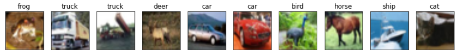
classes = ("plane", "car", "bird", "cat", "deer", "dog", "frog", "horse", "ship", "truck")

Now let's divide all images 255, which will rescale them from 0-255 to 0-1. We'll also convert them for ints to floats, which makes the computations more convenient.

X_train = X_train.astype("float32") / 255
X_test = X_test.astype("float32") / 255

Let's pick the first 10 images from our training set and plot them so we get an idea of what we are dealing with.

Finally, we convert the NumPy arrays that currently hold the images into PyTorch tensors, and we send them to the appropriate device (GPU if CUDA is available and normal memory otherwise).

X_train = torch.tensor(X_train, device=device).permute(0, 3, 1, 2).float()
y_train = torch.tensor(y_train.flatten(), device=device)

Here is the definition of our network. You see that it comprises 2 convolutional layers, 2 pooling layers, a batch normalization layer (to stabilize learning), and three fully connected layers that perform linear transformation.

class Net(nn.Module):
    def __init__(self):
        super().__init__()
        self.conv1 = nn.Conv2d(3, 6, 5)
        self.pool = nn.MaxPool2d(2, 2)
        self.conv2 = nn.Conv2d(6, 16, 5)
        self.batch_norm = nn.BatchNorm2d(16)
        self.fc1 = nn.Linear(16 * 5 * 5, 120)
        self.fc2 = nn.Linear(120, 84)
        self.fc3 = nn.Linear(84, 10)
        

    def forward(self, x):
        x = self.pool(F.relu(self.conv1(x)))
        x = self.pool(F.relu(self.conv2(x)))
        x = self.batch_norm(x)
        
        x = torch.flatten(x, 1) # flatten all dimensions except batch
        x = F.relu(self.fc1(x))
        x = F.relu(self.fc2(x))
        x = self.fc3(x)
        return x

net = Net()
net.to(device)

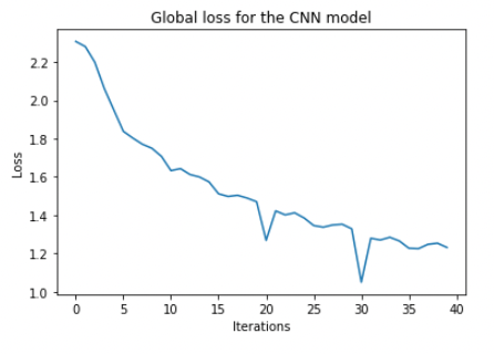
We can plot the training loss and confirm that it is decreasing with training.

fig = plt.figure(figsize=(6,4))
plt.plot(loss_hist)
plt.xlabel("Iterations")
plt.ylabel("Loss")
plt.title("Global loss for the CNN model")
plt.show()

Now let's test the model with some unseen data. We'll make predictions using the hold-out set, plot the first ten images and their respective predicted labels.

outputs = net(torch.tensor(X_test, device=device).permute(0, 3, 1, 2).float())
_, predicted = torch.max(outputs, 1)
fig, ax = plt.subplots(1,10,figsize=(15,2))

for i in range(10):
    ax[i].imshow(X_test[i])
    ax[i].axes.xaxis.set_ticks([])
    ax[i].axes.yaxis.set_ticks([])
    ax[i].title.set_text(classes[predicted[i]])
plt.show()

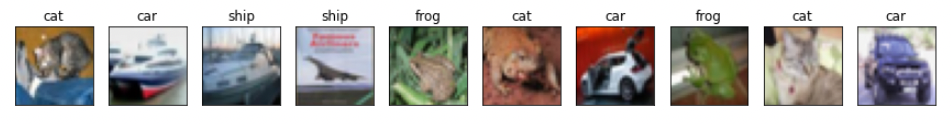
Not too bad, overall, given the simple network architecture and the fact that we didn't spend any time on hyperparameter tuning.

Summary

In this article we introduced Convolutional Neural Networks (CNNs) and provided some intuition on how they extract features and reduce dimensionality. CNNs are predominantly used to address computer vision problems, but they have also being applied to other machine learning domains:

• Recommender systems - CNNs are often used in recommender systems (see Yang et al., 2019; Krupa et al., 2020), and are especially good at handling unstructured data (e.g. video and images). They are good feature extractors and can help alleviate the cold start problem.
• Natural Language Processing - CNNs can be used for sentiment analysis and question classification (Kim, 2014), text classification (Zhang, Zhao, and LeCun, 2015), machine translation ( Gehring et al., 2016), and others
• Time Series Analysis (Lei and Wu, 2020) and others

If you'd like to explore the sample code from this article, please sign up for a free Domino account and you'll get instantaneous access to a notebook and a Python script that you can experiment with. The name of the project is sample-project-2_GPU-trained-CNNs, and it will automatically appear in the Your Projects section.

References

Krupa, K S et al. “Emotion aware Smart Music Recommender System using Two Level CNN.” 2020 Third International Conference on Smart Systems and Inventive Technology (ICSSIT) (2020): 1322-1327. https://ieeexplore.ieee.org/document/9214164

Dan Yang, Jing Zhang, Sifeng Wang, XueDong Zhang, "A Time-Aware CNN-Based Personalized Recommender System", Complexity, vol. 2019, Article ID 9476981, 11 pages, 2019. https://doi.org/10.1155/2019/9476981

Kim, Yoon. 2014. Convolutional Neural Networks for Sentence Classification. https://www.aclweb.org/anthology/D14-1181.pdf.

Zhang, Xiang, Junbo Jake Zhao, and Yann LeCun. 2015. Character-Level Convolutional Networks for Text Classification. https://papers.nips.cc/paper/5782-character-level-convolutional-networks-for-text-classification.pdf

Jonas Gehring, Michael Auli, David Grangier, Yann N. Dauphin. 2016. A Convolutional Encoder Model for Neural Machine Translation, https://arxiv.org/abs/1611.02344

Lei, Yuxia and Zhongqiang Wu. “Time series classification based on statistical features.” EURASIP Journal on Wireless Communications and Networking 2020 (2020): 1-13. https://www.semanticscholar.org/paper/Time-series-classification-based-on-statistical-Lei-Wu/529f639407cb6b3b591b69a93de9c7124c826fa7