HyperOpt: Bayesian Hyperparameter Optimization

Introduction

Feature engineering and hyperparameter optimization are two important model building steps. Over the years, I have debated with many colleagues as to which step has more impact on the accuracy of a model. While this debate has not yet been settled, it is evident that hyperparameter optimization takes up considerable computational resources and time during the model building phase of the Machine Learning lifecycle. There are six main approaches to hyperparameter optimization which include manual search, grid search, random search, evolutionary algorithms, Bayesian optimization, and gradient based methods.

While it has been empirically and theoretically shown that popular methods like random search are more efficient than grid search, these approaches are not intelligent in how they explore the search space of hyperparameters. Training AI needs to become more energy conscious, and hyperparameter optimization is a suitable area to focus on as it is compute intensive. Since Bayesian optimization is not a brute force algorithm—as compared to manual, grid and random search—it is a good choice for performing hyperparameter optimization in an efficient manner while not compromising the quality of the results.

The HyperOpt package, developed with support from leading government, academic and private institutions, offers a promising and easy-to-use implementation of a Bayesian hyperparameter optimization algorithm. In the remainder of this article, we will cover how to perform hyperparameter optimization using a sequential model-based optimization (SMBO) technique implemented in the HyperOpt Python package.

Bayesian Sequential Model-based Optimization (SMBO) using HyperOpt

Sequential model-based optimization is a Bayesian optimization technique that uses information from past trials to inform the next set of hyperparameters to explore, and there are two variants of this algorithm used in practice:one based on the Gaussian process and the other on the Tree Parzen Estimator. The HyperOpt package implements the Tree Parzen Estimator algorithm to perform optimization which is described in the section below.

Understanding the Tree Parzen Estimator

The Tree Parzen Estimator replaces the generative process of choosing parameters from the search space in a tree like fashion with a set of non parametric distributions. It replaces choices for parameter distributions with either a truncated Gaussian mixture,an exponentiated truncated Gaussian mixture or a re-weighted categorical to form two densities—one density for the loss function, where the loss is below a certain threshold, and another for a density where the loss function is above a certain threshold for values in the hyperparameter space. With each sampled configuration from the densities that is evaluated, the densities are updated to make them represent the true loss surface more precisely.

How to Optimize the Hyperparameters

Here we demonstrate how to optimize the hyperparameters for a logistic regression, random forest, support vector machine, and a k-nearest neighbour classifier from the Jobs dashboard in Domino. Apart from starting the hyperparameter jobs, the logs of the jobs and the results of the best found hyperparameters can also be seen in the Jobs dashboard.

In order to run the hyperparameter optimization jobs, we create a Python file (hpo.py) that takes a model name as a parameter and start the jobs using the Run option in the Jobs dashboard in Domino.

Step 1: Install the required dependencies for the project by adding the following to your Dockerfile

RUN pip install numpy==1.13.1RUN pip install hyperoptRUN pip install scipy==0.19.1

Step 2 : Create a Python file and load the required libraries

from hyperopt import hp, tpe, fmin, Trials, STATUS_OK
from sklearn import datasets
from sklearn.neighbors import KNeighborsClassifier
from sklearn.svm import SVC
from sklearn.linear_model import LogisticRegression
from sklearn.ensemble.forest import RandomForestClassifier
from sklearn.preprocessing import scale, normalize
from sklearn.model_selection import cross_val_score
import numpy as np
import pandas as pd
import matplotlib.pyplot as plt

Step 3 : Specify the algorithms for which you want to optimize hyperparameters

models = {
'logistic_regression' : LogisticRegression,
'rf' : RandomForestClassifier,
'knn' : KNeighborsClassifier,
'svc' : SVC}

Step 4: Setup the hyperparameter space for each of the algorithms

def search_space(model):
    model = model.lower()
    space = {}
    if model == 'knn':
        space = {
            'n_neighbors': hp.choice('n_neighbors', range(1,100)),
            'scale': hp.choice('scale', [0, 1]),
            'normalize': hp.choice('normalize', [0, 1]),
            }
    elif model == 'svc':
        space = {
            'C': hp.uniform('C', 0, 20),
            'kernel': hp.choice('kernel', ['linear', 'sigmoid', 'poly', 'rbf']),
            'gamma': hp.uniform('gamma', 0, 20),
            'scale': hp.choice('scale', [0, 1]),
            'normalize': hp.choice('normalize', [0, 1]),
            }
    elif model == 'logistic_regression':
        space = {
            'warm_start' : hp.choice('warm_start', [True, False]),
            'fit_intercept' : hp.choice('fit_intercept', [True, False]),
            'tol' : hp.uniform('tol', 0.00001, 0.0001),
            'C' : hp.uniform('C', 0.05, 3),
            'solver' : hp.choice('solver', ['newton-cg', 'lbfgs', 'liblinear']),
            'max_iter' : hp.choice('max_iter', range(100,1000)),
            'scale': hp.choice('scale', [0, 1]),
            'normalize': hp.choice('normalize', [0, 1]),
            'multi_class' : 'auto',
            'class_weight' : 'balanced'
                }
    elif model == 'rf':
    space = {'max_depth': hp.choice('max_depth', range(1,20)),
    'max_features': hp.choice('max_features', range(1,3)),
    'n_estimators': hp.choice('n_estimators', range(10,50)),
    'criterion': hp.choice('criterion', ["gini", "entropy"]),
        }
    space['model'] = model
    return space

Step 5 : Define the loss metric for the model

In this step, we have defined a 5 fold cross-validation score as the loss, and since HyperOpt’s optimizer performs minimization, we add a negative sign to the cross-validation score.

def get_acc_status(clf,X_,y):
    acc = cross_val_score(clf, X_, y, cv=5).mean()
    return {'loss': -acc, 'status': STATUS_OK}

Step 6 : Construct the objective function for the HyperOpt optimizer

In this step, we pass in the hyperparameters and return the value computed by the loss function for a set of hyperparameters.

def obj_fnc(params):
    model = params.get('model').lower()
    X_ = scale_normalize(params,X[:])
    del params['model']
    clf = models[model](**params)
    return(get_acc_status(clf,X_,y))

Step 7 : Create a trial object to store the results of each evaluation and print the best result found

hypopt_trials = Trials()
best_params = fmin(obj_fnc, search_space(model), algo=tpe.suggest,
max_evals=1000, trials= hypopt_trials)
print(best_params)
print(hypopt_trials.best_trial['result']['loss'])

Step 8 : Write the model name, accuracy and best hyperparameters found to dominostats.json

Once the data is written to dominostats.json, the results will be visible in the Jobs dashboard in Domino.

with open('dominostats.json', 'w') as f:
    f.write(json.dumps({"Algo": model, "Accuracy":
    hypopt_trials.best_trial['result']['loss'],"Best params" : best_params}))

Step 9 : Start the hyperparameter optimization jobs from the Jobs dashboard

Steps 9 & 10 are specific to Domino users, but if you aren't using Domino you can still execute the hpo.py script and inspect the results manually.

In Domino, navigate to the Jobs dashboard using the navigation panel on the left hand side and click on the Run option to execute hpo.py with the model name as a parameter.

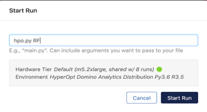
Execute the hyperparameter optimization jobs

Step 10 : View the results on the Jobs dashboard

The results show that the support vector classifier has the best accuracy (0.993—and it was able to find a good separation hyperplane fairly quickly) whereas the random forest has the least accuracy (0.966).

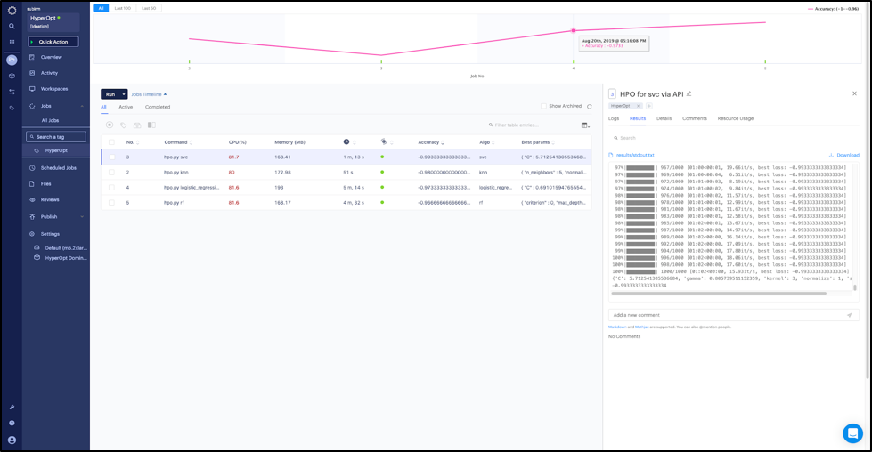
Jobs dashboard with results of the different hyperparameter optimization runs

Conclusion

Bayesian hyperparameter optimization is an intelligent way to perform hyperparameter optimization. It helps save on computational resources and time and usually shows results at par, or better than, random search. The HyperOpt library makes it easy to run Bayesian hyperparameter optimization without having to deal with the mathematical complications that usually accompany Bayesian methods. HyperOpt also has a vibrant open source community contributing helper packages for sci-kit models and deep neural networks built using Keras.

In addition, when executed in Domino using the Jobs dashboard, the logs and results of the hyperparameter optimization runs are available in a fashion that makes it easy to visualize, sort and compare the results.