N-shot and Zero-shot learning with Python
Dr Behzad Javaheri2022-04-28 | 12 min read

Introduction
In a previous post we talked about how advances in deep learning neural networks have allowed significant improvements in learning performance, resulting in their dominance in some areas like computer vision. We also pointed out some of the roadblocks that prevent wider adoption of complex machine learning models. Training a model in many instances requires large, annotated datasets, which may not always be available in some domains (for example the medical field). In addition, in multiclass classifications, class imbalance poses an additional challenge. Moreover, a model trained on one dataset may not perform similarly well on a separate dataset due to differences in input features and feature distribution. To top it off, the growing computational requirements of state-of-the-art models often prevent us from training complex models from scratch. To circumvent these issues, and leverage the power of neural networks, one simple approach is to utilise an increasingly popular transfer function approach. This function allows building new models using weights from pre-trained models, which have already been trained on one task (e.g., classification) and one dataset (e.g., ImageNet as one of the largest open-source datasets), and use the new models on a similar task and unseen dataset.
The intuition behind transfer learning is that if datasets in two problems contain similar data points, their feature representations are also similar and thus the weights obtained from one training can be used in solving subsequent similar problems rather than using random weights and model training from scratch. The pre-trained models can be fitted quicker on the second task as they already contain training weights from the first task. We already showed the use of pre-trained models (via HuggingFace) for solving NLP problems. Now let's see how we can apply transfer learning in cases where examples are scarce or no labelled data is available at all.
What is N-shot learning?
The availability of large datasets, including ImageNet with more than 1000 classes, access to GPUs and cloud computing, and advances in deep learning have allowed the development of highly accurate models to solve problems across many domains. These models as described previously can be re-used via transfer learning to solve problems with similar data.
The main requirement for transfer learning is availability and access to large scale data for training. This is not always possible, and some real-world problems suffer from data scarcity. For example, there are around 369,000 vascular plant species that are known flowering plants. One of these is Corpse Lily which is the largest known flower. This is a rare plant and therefore in a given computer vision classification task, there will be far fewer images of this plant compared to more common flowering plants.
Variants of the transfer learning approach have been designed to address this key issue around data availability, alongside other challenges like training time and high infrastructure costs. Some of these variants are aiming implement learning with a handful of examples, in an attempt to mimic the human process. N-shot learning (NSL) aims to build models using the training set \(D_{train}\) that consists of input \(x_i\)’s together with their output \(y_i\)’s [1-3]. This approach has been utilised to solve a variety of problems including object recognition [1], image classification [4] and sentiment classification [5]. In classification tasks, the algorithm learns a classifier \(h\) to predict label \(y_i\) for the corresponding \(x_i\). Usually, one considers the N -way-K-shot classification , in which \(D_train\) contains \(I = KN\) examples from \(N\) classes each with \(K\) examples. Few-shot regression estimates a regression function \(h\) given only a few input-output example pairs sampled from that function, where output \(y_i\) is the observed value of the dependent variable \(y\), and \(x_i\) is the input which records the observed value of the independent variable \(x\). Moreover, NSL has been utilised with reinforcement learning with only limited trajectories of state-action pairs to identify an optimal policy [6, 7].
A shot is essentially an example used for training, with \(N\) defining the number of data points. There are three main variants of NSL: few-shot, one-shot and zero-shot. Few-shot is the most flexible variant with a few data points for training with zero-shot being the most restrictive with no datapoint for training. We will provide additional background and examples for zero-shot learning.
What is Zero-shot learning?
Zero-shot learning is a variant of transfer learning with no labelled examples to learn during training. This method uses additional information to comprehend the unseen data. In this method, three variables are learned. These are the input variable \(x\), the output variable \(y\), and the additional random variable that describes the task \(T\). The model is thus trained to learn the conditional probability distribution of \(P(y | x, T)\) [8].
Here we will use the task-aware representation of sentences (TARS) which was introduced by Halder et al. (2020) as a simple and effective method for few-shot and even zero-shot learning for text classification. This means you can classify text without many training examples. This model is implemented in Flair by the TARSClassifier class [9].
Below we will utilise TARS for zero-shot classification and Named Entity Recognition (NER) tasks. In this tutorial, we will show you different ways of using TARS. We will provide input texts and labels and the predict_zero_shot method of TARS will try to match one of these labels to the text.
Using Zero-shot learning for text classification
# Loading pre-trained TARS model for English
tars: TARSClassifier = TARSClassifier.load('tars-base')

# the sentence for classification
sentence = Sentence("The 2020 United States presidential election was the 59th quadrennial presidential election, held on Tuesday, November 3, 2020")

classes = ["sports", "politics", "science", "art"]

# predict the class of the sentence
tars.predict_zero_shot(sentence, classes)

# Print sentence with predicted labels
print("\n",sentence)
The out prints the class which the TARS Classifier identifies:
Sentence: "The 2020 United States presidential election was the 59th quadrennial presidential election , held on Tuesday , November 3 , 2020" [− Tokens: 21 − Sentence-Labels: 'sports-politics-science-art': [politics (1.0)]”Using Zero-shot learning for Named Entity Recognition (NER)
# 1. Load zero-shot NER tagger
tars = TARSTagger.load('tars-ner')

# 2. Prepare some test sentences
sentences = [
    Sentence("The Humboldt University of Berlin is situated near the Spree in Berlin, Germany"),
    Sentence("Bayern Munich played against Real Madrid"),
    Sentence("I flew with an Airbus A380 to Peru to pick up my Porsche Cayenne"),
    Sentence("Game of Thrones is my favorite series"),
]

# 3. Define some classes of named entities such as "soccer teams", "TV shows" and "rivers"
labels = ["Soccer Team", "University", "Vehicle", "River", "City", "Country", "Person", "Movie", "TV Show"]
tars.add_and_switch_to_new_task('task 1', labels, label_type='ner')

# 4. Predict for these classes and print results
for sentence in sentences:
    tars.predict(sentence)
    print(sentence.to_tagged_string("ner"))
The output printed below identifies NER associated with each entity without the model being explicitly trained to identify it. For example, we are finding entity classes such as "TV show" (Game of Thrones), "vehicle" (Airbus A380 and Porsche Cayenne), "soccer team" (Bayern Munich and Real Madrid) and "river" (Spree)
The Humboldt <B-University> University <I-University> of <I-University> Berlin <E-University> is situated near the Spree <S-River> in Berlin <S-City> , Germany <S-Country>
Bayern <B-Soccer Team> Munich <E-Soccer Team> played against Real <B-Soccer Team> Madrid <E-Soccer Team>
I flew with an Airbus <B-Vehicle> A380 <E-Vehicle> to Peru <S-City> to pick up my Porsche <B-Vehicle> Cayenne <E-Vehicle>
Game <B-TV Show> of <I-TV Show> Thrones <E-TV Show> is my favorite series
What is One-shot learning?
The term, one-shot was coined in a seminal paper by Fei-Fei et al., (2006) proposing a variation on a Bayesian framework for representation learning for object categorisation [1]. One-shot learning allows model learning from one instance of the datapoint. This enables models to exhibit learning behaviour similar to humans. For example, once a child observes the overall shape and colour of an apple, the child can easily identify another apple. In humans, this could be achieved with one or a few data points. This ability is extremely helpful to solve real-world problems where access to many labelled data points is not always possible.
One-shot learning is usually implemented based on similarity, learning and data. In this example we will use Siamese Networks (for discriminating two unseen classes) which is based on similarity. A Siamese Neural Network is a class of neural network architectures that contain two or more identical subnetworks. Identical here means that they have the same configuration with the same parameters and weights. The two subnetwork output an encoding to calculate the difference between the two inputs. The Siamese network's objective is to classify if the two inputs are the same or different using a similarity score.
Let's create a simple one-shot learning example using the MNIST Dataset and Keras.
We start by importing all the needed Python modules, loading the MNIST dataset, and normalising and reshaping the data.
import numpy as np
from keras.datasets import mnist
import matplotlib.pyplot as plt
from tensorflow.keras import layers, models

# import keras as ks
import tensorflow as tf
import pickle
from tensorflow.keras.layers import Activation
from tensorflow.keras.layers import Flatten
from tensorflow.keras.layers import Dense
from tensorflow.keras.layers import Reshape
from tensorflow.keras.layers import Input
from tensorflow.keras.models import Model
from tensorflow.keras.layers import Dot
from tensorflow.keras.layers import Lambda
from tensorflow.keras import backend as K

# import keras
import random
import tensorflow_addons as tfa

import matplotlib.pyplot as plt
from matplotlib.colors import ListedColormap

(X_train, Y_train), (X_test, Y_test) = mnist.load_data()

# We need to normalise the training and testing subsets
X_train = X_train.astype('float32')
X_train /= 255
X_train = X_train.reshape((len(X_train), np.prod(X_train.shape[1:])))
X_test = X_test.astype('float32')
X_test /= 255
X_test = X_test.reshape((len(X_test), np.prod(X_test.shape[1:])))

# Printing data shape
print("The shape of X_train and Y_train: {} and {} ".format(X_train.shape, Y_train.shape))
print("The shape of X_test and Y_test: {} and {} ".format(X_test.shape, Y_test.shape))
The shape of X_train and Y_train: (60000, 784) and (60000,)
The shape of X_test and Y_test: (10000, 784) and (10000,)
Next, we need to create the image pairs. Since the siamese network has two input channels, we must arrange the input data into pairs. A positive pairs will contain two images that belong to the same class and a negative pair will contain two images that belong to different classes.
class Pairs:
    def makePairs(self, x, y):
        num_classes = 10
        digit_indices = [np.where(y == i)[0] for i in range(num_classes)]

        pairs = list()
        labels = list()

        for idx1 in range(len(x)):
            x1 = x[idx1]
            label1 = y[idx1]
            idx2 = random.choice(digit_indices[label1])
            x2 = x[idx2]

            labels += list([1])
            pairs += [[x1, x2]]

            label2 = random.randint(0, num_classes-1)
            while label2 == label1:
                label2 = random.randint(0, num_classes-1)

            idx2 = random.choice(digit_indices[label2])
            x2 = x[idx2]

            labels += list([0])
            pairs += [[x1, x2]]

        return np.array(pairs), np.array(labels)
Let's construct the pairs.
p = Pairs()
pairs_train, labels_train = p.makePairs(X_train, Y_train)
pairs_test, labels_test = p.makePairs(X_test, Y_test)
labels_train = labels_train.astype('float32')
labels_test = labels_test.astype('float32')
Next, we define the distance metric (we use Euclidean distance), the loss function (contrastive loss), and a function for calculating the model accuracy.
def euclideanDistance(v):
    x, y = v
    sum_square = K.sum(K.square(x - y), axis=1, keepdims=True)
    return K.sqrt(K.maximum(sum_square, K.epsilon()))

def eucl_dist_output_shape(shapes):
    shape1, shape2 = shapes
    return (shape1[0], 1)

def contrastive_loss(y_original, y_pred):
    sqaure_pred = K.square(y_pred)
    margin = 1
    margin_square = K.square(K.maximum(margin - y_pred, 0))
    return K.mean(y_original * sqaure_pred + (1 - y_original) * margin_square)

def compute_accuracy(y_original, y_pred):
    pred = y_pred.ravel() < 0.5
    return np.mean(pred == y_original)

def accuracy(y_original, y_pred):
    return K.mean(K.equal(y_original, K.cast(y_pred < 0.5, y_original.dtype)))
We can now move onto building and compiling the model. We'll use (786,) input layer, which corresponds to a 28x28 pixels matrix, followed by three fully connected layers with ReLU activation, and two L2 normalisation layers. We'll compile the model and print a summary of its layers and parameters.
input = Input(shape=(784,))
x = Flatten()(input)
x = Dense(64, activation='relu')(x)
x = Dense(128, activation='relu')(x)
x = Dense(256, activation='relu')(x)
x = Lambda(lambda  x: K.l2_normalize(x,axis=1))(x)
x = Lambda(lambda  x: K.l2_normalize(x,axis=1))(x)
dense = Model(input, x)

input1 = Input(shape=(784,))
input2 = Input(shape=(784,))
dense1 = dense(input1)
dense2 = dense(input2)

distance = Lambda(euclideanDistance, output_shape=eucl_dist_output_shape)([dense1, dense2])
model = Model([input1, input2], distance)

# Compiling and printing a summary of model architecture
model.compile(loss = contrastive_loss, optimizer="adam", metrics=[accuracy])
model.summary()
Model: "functional_47"
__________________________________________________________________________________________________
Layer (type) Output Shape Param # Connected to
==================================================================================================
input_36 (InputLayer) [(None, 784)] 0
__________________________________________________________________________________________________
input_37 (InputLayer) [(None, 784)] 0
__________________________________________________________________________________________________
functional_45 (Functional) (None, 256) 91584 input_36[0][0]
input_37[0][0]
__________________________________________________________________________________________________
lambda_35 (Lambda) (None, 1) 0 functional_45[0][0]
functional_45[1][0]
==================================================================================================
Total params: 91,584
Trainable params: 91,584
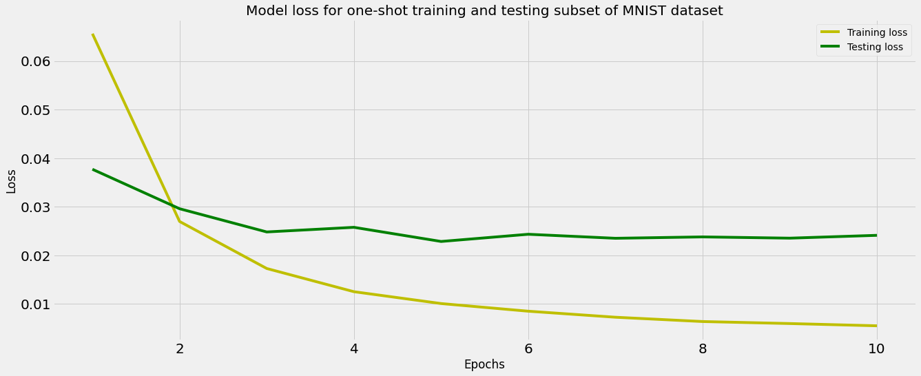
Non-trainable params: 0We can now train the network for 10 epochs and capture the changes in the training and test loss over the period of training.
# Prediction and printing accuracy
y_pred_te = model.predict([pairs_test[:, 0], pairs_test[:, 1]])
te_acc = compute_accuracy(labels_test, y_pred_te)
print("The accuracy obtained on testing subset: {}".format(te_acc*100))
The accuracy obtained on testing subset: 97.13000000000001
We can also plot the two losses over time and inspect the plot for signs of overfitting.
# Plotting training and testing loss
plt.figure(figsize=(20,8));
history_dict = history.history;
loss_values = history_dict['loss'];
val_loss_values = history_dict['val_loss'];
epochs = range(1, (len(history.history['val_accuracy']) + 1));
plt.plot(epochs, loss_values, 'y', label='Training loss');
plt.plot(epochs, val_loss_values, 'g', label='Testing loss');
plt.title('Model loss for one-shot training and testing subset of MNIST dataset');
plt.xlabel('Epochs');
plt.ylabel('Loss');
plt.legend();
Conclusion
Transfer learning and its variants including one-shot and zero-shot learning are aiming to address some of the fundamental obstacles like data scarcity faced in machine learning applications. The ability to learn intelligently from fewer data makes artificial intelligence similar to human learning and paves the way for wider adoption.
References
[1] L. Fei-Fei, R. Fergus, and P. Perona, "One-shot learning of object categories," IEEE transactions on pattern analysis and machine intelligence, vol. 28, no. 4, pp. 594-611, 2006.
[2] E. G. Miller, N. E. Matsakis, and P. A. Viola, "Learning from one example through shared densities on transforms," in Proceedings IEEE Conference on Computer Vision and Pattern Recognition. CVPR 2000 (Cat. No. PR00662), 2000, vol. 1: IEEE, pp. 464-471.
[3] C. M. Bishop and N. M. Nasrabadi, Pattern recognition and machine learning (no. 4). Springer, 2006.
[4] O. Vinyals, C. Blundell, T. Lillicrap, and D. Wierstra, "Matching networks for one shot learning," Advances in neural information processing systems, vol. 29, 2016.
[5] M. Yu et al., "Diverse few-shot text classification with multiple metrics," arXiv preprint arXiv:1805.07513, 2018.
[6] A. Grover, M. Al-Shedivat, J. Gupta, Y. Burda, and H. Edwards, "Learning policy representations in multiagent systems," in International conference on machine learning, 2018: PMLR, pp. 1802-1811.
[7] Y. Duan et al., "One-shot imitation learning," Advances in neural information processing systems, vol. 30, 2017.
[8] I. Goodfellow, Y. Bengio, and A. Courville, Deep learning. MIT press, 2016.
[9] K. Halder, A. Akbik, J. Krapac, and R. Vollgraf, "Task-aware representation of sentences for generic text classification," in Proceedings of the 28th International Conference on Computational Linguistics, 2020, pp. 3202-3213.

RELATED TAGS
SHARE


Subscribe to the Domino Newsletter
Receive data science tips and tutorials from leading Data Science leaders, right to your inbox.
By submitting this form you agree to receive communications from Domino related to products and services in accordance with Domino's privacy policy and may opt-out at anytime.