
This article covers causal relationships and includes a chapter excerpt from the book Machine Learning in Production: Developing and Optimizing Data Science Workflows and Applications by Andrew Kelleher and Adam Kelleher.
Introduction
As data science work is experimental and probabilistic in nature, data scientists are often faced with making inferences. This may require a shift in mindset, particularly if moving from "traditional statistical analysis to causal analysis of multivariate data". As Domino is committed to providing the platform and tools data scientists need to accelerate their work, we reached out to Addison-Wesley Professional (AWP) Pearson for permission to excerpt "Causal Inference" from the book, Machine Learning in Production: Developing and Optimizing Data Science Workflows and Applications by Andrew Kelleher and Adam Kelleher.

Chapter Introduction: Causal Inference
We’ve introduced [in the book] a couple of machine-learning algorithms and suggested that they can be used to produce clear, interpretable results. You’ve seen that logistic regression coefficients can be used to say how much more likely an outcome will occur in conjunction with a feature (for binary features) or how much more likely an outcome is to occur per unit increase in a variable (for real-valued features). We’d like to make stronger statements. We’d like to say “If you increase a variable by a unit, then it will have the effect of making an outcome more likely.”
These two interpretations of a regression coefficient are so similar on the surface that you may have to read them a few times to take away the meaning. The key is that in the first case, we’re describing what usually happens in a system that we observe. In the second case, we’re saying what will happen if we intervene in that system and disrupt it from its normal operation.
After we go through an example, we’ll build up the mathematical and conceptual machinery to describe interventions. We’ll cover how to go from a Bayesian network describing observational data to one that describes the effects of an intervention. We’ll go through some classic approaches to estimating the effects of interventions, and finally we’ll explain how to use machine-learning estimators to estimate the effects of interventions.
If you imagine a binary outcome, such as “I’m late for work,” you can imagine some features that might vary with it. Bad weather can cause you to be late for work. Bad weather can also cause you to wear rain boots. Days when you’re wearing rain boots, then, are days when you’re more likely be late for work. If you look at the correlation between the binary feature “wearing rain boots” and the outcome “I’m late for work,” you’ll find a positive relationship. It’s nonsense, of course, to say that wearing rain boots causes you to be late for work. It’s just a proxy for bad weather. You’d never recommend a policy of “You shouldn’t wear rain boots, so you’ll be late for work less often.” That would be reasonable only if “wearing rain boots” was causally related to “being late for work.” As an intervention to prevent lateness, not wearing rain boots doesn’t make any sense.
In this chapter, you’ll learn the difference between correlative (rain boots and lateness) and causal (rain and lateness) relationships. We’ll discuss the gold standard for establishing causality: an experiment. We’ll also cover some methods to discover causal relationships in cases when you’re not able to run an experiment, which happens often in realistic settings.
13.2 Experiments
The case that might be familiar to you is an AB test. You can make a change to a product and test it against the original version of the product. You do this by randomly splitting your users into two groups. The group membership is denoted by D, where D = 1 is the group that experiences the new change (the test group), and D = 0 is the group that experiences the original version of the product (the control group). For concreteness, let’s say you’re looking at the effect of a recommender system change that recommends articles on a website. The control group experiences the original algorithm, and the test group experiences the new version. You want to see the effect of this change on total pageviews, Y.
You’ll measure this effect by looking at a quantity called the average treatment effect (ATE). The ATE is the average difference in the outcome between the test and control groups,
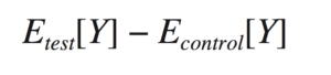
or
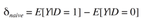
This is the “naive” estimator for the ATE since here we’re ignoring everything else in the world. For experiments, it’s an unbiased estimate for the true effect.
A nice way to estimate this is to do a regression. That lets you also measure error bars at the same time and include other covariates that you think might reduce the noise in Y so you can get more precise results. Let’s continue with this example.
import numpy as np
import pandas as pd

N = 1000
x = np.random.normal(size=N)
d = np.random.binomial(1., 0.5, size=N)
y = 3. * d + x + np.random.normal()
X = pd.DataFrame({'X': x, 'D': d, 'Y': y})
Here, we’ve randomized D to get about half in the test group and half in the control. X is some other covariate that causes Y, and Y is the outcome variable. We’ve added a little extra noise to Y to just make the problem a little noisier.
You can use a regression model
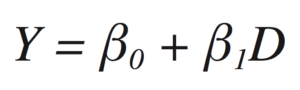
to estimate the expected value of Y, given the covariate D, as
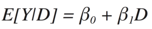
The β0 piece will be added to E[Y|D] for all values of D (i.e., 0 or 1). The β1 part is added only when D = 1 because when D = 0, it’s multiplied by zero. That means
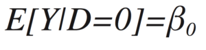
when D=0 and
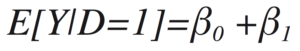
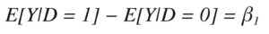
when D=1. Thus, the β1 coefficientis going to be the difference in average Y values between the D = 1 group and the D = 0 group,
You can use that coefficient to estimate the effect of this experiment. When you do the regression of Y against D, you get the result in Figure 13.1.
from statsmodels.api import OLS
X['intercept'] = 1.
model = OLS(X['Y'], X[['D', 'intercept']])
result = model.fit()
result.summary()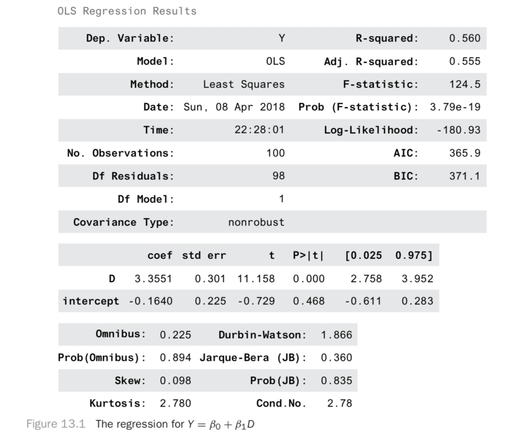
Why did this work? Why is it okay to say the effect of the experiment is just the difference between the test and control group outcomes? It seems obvious, but that intuition will break down in the next section. Let’s make sure you understand it deeply before moving on.
Each person can be assigned to the test group or the control group, but not both. For a person assigned to the test group, you can talk hypothetically about the value their outcome would have had, had they been assigned to the control group. You can call this value Y0 because it’s the value Y would take if D had been set to 0. Likewise, for control group members, you can talk about a hypothetical Y1. What you really want to measure is the difference in outcomes
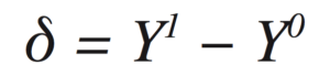
for each person. This is impossible since each person can be in only one group! For this reason, these Y1 and Y0 variables are called potential outcomes.
If a person is assigned to the test group, you measure the outcome Y = Y1. If a person is assigned to the control group, you measure Y = Y0. Since you can’t measure the individual effects, maybe you can measure population level effects. We can try to talk instead about E[Y1] and E[Y0]. We’d like
![E[Y1] and E[Y0]](https://cdn.sanity.io/images/kuana2sp/production-main/4eeebdbcfa0ac4f9f99d09c1981767fb58adbc3a-300x60.png?w=1920&fit=max&auto=format)
and
![E[Y1] and E[Y0]](https://cdn.sanity.io/images/kuana2sp/production-main/1a316f3802f933a2d70118937e8a581f38d4c79c-300x59.png?w=1920&fit=max&auto=format)
but we’re not guaranteed that that’s true. In the recommender system test example, what would happen if you assigned people with higher Y0 pageview counts to the test group? You might measure an effect that’s larger than the true effect!
Fortunately, you randomize D to make sure it’s independent of Y0 and Y1. That way, you’re sure that
and
so you can say that
![E[Y1] and E[Y0]](https://cdn.sanity.io/images/kuana2sp/production-main/409aee19bb2e02ce13ee3616d877897c55d23931-1024x83.png?w=1920&fit=max&auto=format)
When other factors can influence assignment, D, then you can no longer be sure you have correct estimates! This is true in general when you don’t have control over a system, so you can’t ensure D is independent of all other factors.
In the general case, D won’t just be a binary variable. It can be ordered, discrete, or continuous. You might wonder about the effect of the length of an article on the share rate, about smoking on the probability of getting lung cancer, of the city you’re born in on future earnings, and so on.
Just for fun before we go on, let’s see something nice you can do in an experiment to get more precise results. Since we have a co-variate, X, that also causes Y, we can account for more of the variation in Y. That makes our predictions less noisy, so our estimates for the effect of D will be more precise! Let’s see how this looks. We regress on both D and X now to get Figure 13.2.
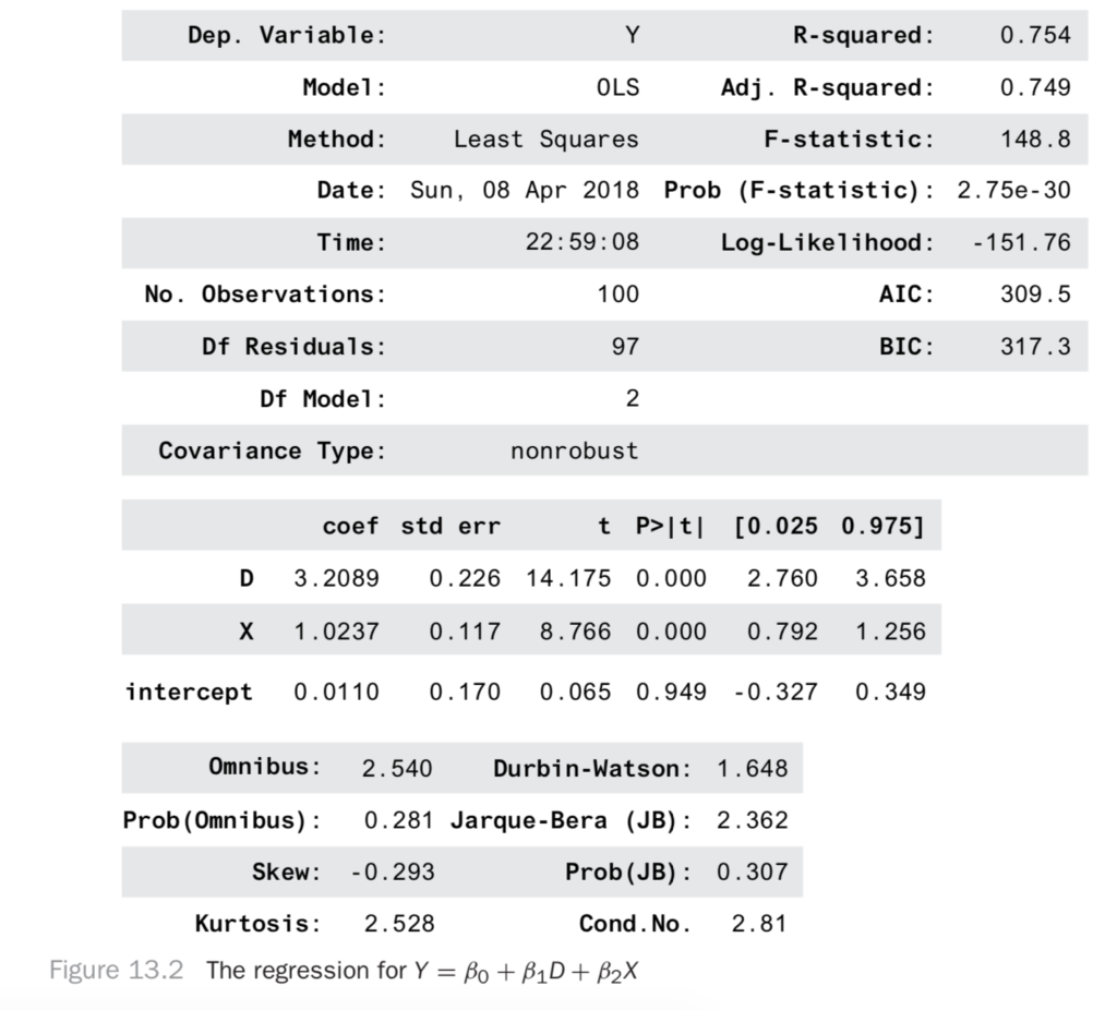
Notice that the R2 is much better. Also, notice that the confidence interval for D is much narrower! We went from a range of 3.95 − 2.51 = 1.2 down to 3.65 − 2.76 = 0.89. In short, finding covariates that account for the outcome can increase the precision of your experiments!
13.3 Observation: An Example
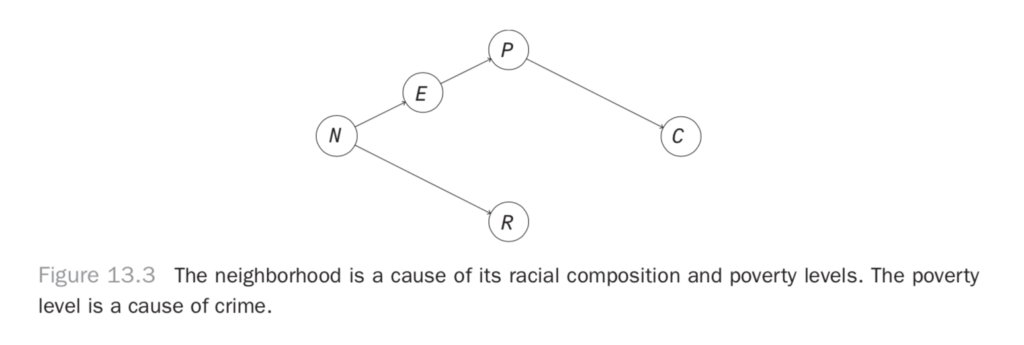
Let’s look at an example of what happens when you don’t make your cause independent of everything else. We’ll use it to show how to build some intuition for how observation is different from intervention. Let’s look at a simple model for the correlation between race, poverty, and crime in a neighborhood. Poverty reduces people’s options in life and makes crime more likely. That makes poverty a cause of crime. Next, neighborhoods have a racial composition that can persist over time, so the neighborhood is a cause of racial composition. The neighborhood also determines some social factors, like culture and education, and so can be a cause of poverty. This gives us the causal diagram in Figure 13.3.
Here, there is no causal relationship between race and crime, but you would find them to be correlated in observational data. Let’s simulate some data to examine this.
N = 10000
neighborhood = np.array(range(N))
industry = neighborhood % 3
race = ((neighborhood % 3
+ np.random.binomial(3, p=0.2, size=N))) % 4
income = np.random.gamma(25, 1000*(industry + 1))
crime = np.random.gamma(100000. / income, 100, size=N)
X = pd.DataFrame({'$R$': race, '$I$': income, '$C$': crime,
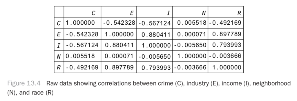
'$E$': industry, '$N$': neighborhood})Here, each data point will be a neighborhood. There are common historic reasons for the racial composition and the dominant industry in each neighborhood. The industry determines the income levels in the neighborhood, and the income level is inversely related with crime rates.
If you plot the correlation matrix for this data (Figure 13.4), you can see that race and crime are correlated, even though there is no causal relationship between them!
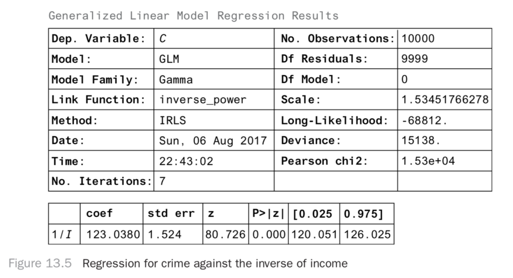
You can take a regression approach and see how you can interpret the regression coefficients. Since we know the right model to use, we can just do the right regression, which gives the results in Figure 13.5.
from statsmodels.api import GLM
import statsmodels.api as sm
X['$1/I$'] = 1. / X['$I$']
model = GLM(X['$C$'], X[['$1/I$']], family=sm.families.Gamma())
result = model.fit()
result.summary()
From this you can see that when 1/I increases by a unit, the number of crimes increases by 123 units. If the crime units are in crimes per 10,000 people, this means 123 more crimes per 10,000 people.
This is a nice result, but you’d really like to know whether the result is causal. If it is causal, that means you can design a policy intervention to exploit the relationship. That is, you’d like to know if people earned more income, everything else held fixed, would there be less crime? If this were a causal result, you could say that if you make incomes higher (independent of everything else), then you can expect that for each unit decrease in 1/I, you’ll see 123 fewer crimes. What is keeping us from making those claims now?
You’ll see that regression results aren’t necessarily causal; let’s look at the relationship between race and crime. We’ll do another regression as shown here:
from statsmodels.api import GLM
import statsmodels.api as sm
races = {0: 'african-american', 1: 'hispanic',
    2: 'asian', 3: 'white'}
X['race'] = X['$R$'].apply(lambda x: races[x])
race_dummies = pd.get_dummies(X['race'])
X[race_dummies.columns] = race_dummies
model = OLS(X['$C$'], race_dummies)
result = model.fit()
result.summary()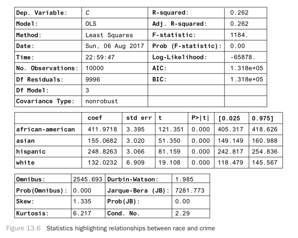
Here, you find a strong correlative relationship between race and crime, even though there’s no causal relationship. You know that if we moved a lot of white people into a black neighborhood (holding income level constant), you should have no effect on crime. If this regression were causal, then you would. Why do you find a significant regression coefficient even when there’s no causal relationship?
In this example, you went wrong because racial composition and income level were both caused by the history of each neighborhood. This is a case where two variables share a common cause. If you don’t control for that history, then you’ll find a spurious association between the two variables. What you’re seeing is a general rule: when two variables share a common cause, they will be correlated (or, more generally, statistically dependent) even when there’s no causal relationship between them.
Another nice example of this common cause problem is that when lemonade sales are high, crime rates are also high. If you regress crime on lemonade sales, you’d find a significant increase in crimes per unit increase in lemonade sales! Clearly the solution isn’t to crack down on lemonade stands. As it happens, more lemonade is sold on hot days. Crime is also higher on hot days. The weather is a common cause of crime and lemonade sales. We find that the two are correlated even though there is no causal relationship between them.
The solution in the lemonade example is to control for the weather. If you look at all days when it is sunny and 95 degrees Fahrenheit, the effect of the weather on lemonade sales is constant. The effect of weather and crime is also constant in the restricted data set. Any variance in the two must be because of other factors. You’ll find that lemonade sales and crime no longer have a significant correlation in this restricted data set. This problem is usually called confounding, and the way to break confounding is to control for the confounder.
Similarly, if you look only at neighborhoods with a specific history (in this case the relevant variable is the dominant industry), then you’ll break the relationship between race and income and so also the relationship between race and crime.
To reason about this more rigorously, let’s look at Figure 13.3. We can see the source of dependence, where there’s a path from N to R and a path from N through E and P to C. If you were able to break this path by holding a variable fixed, you could disrupt the dependence that flows along it. The result will be different from the usual observational result. You will have changed the dependencies in the graph, so you will have changed the joint distribution of all these variables.
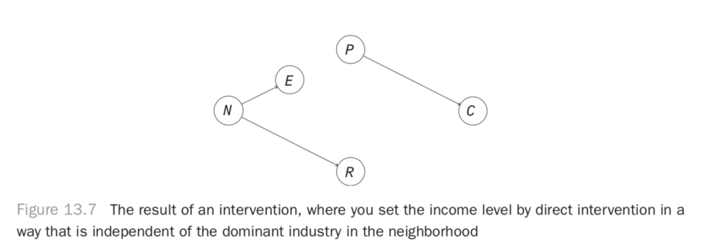
If you intervene to set the income level in an area in a way that is independent of the dominant industry, you’ll break the causal link between the industry and the income, resulting in the graph in Figure 13.7. In this system, you should find that the path that produces dependence between race and crime is broken. The two should be independent.
How can you do this controlling using only observational data? One way is just to restrict to subsets of the data. You can, for example, look only at industry 0 and see how this last regression looks.
X_restricted = X[X['$E$'] == 0]
races = {0: 'african-american', 1: 'hispanic',
    2: 'asian', 3: 'white'}
X_restricted['race'] = X_restricted['$R$'].apply(lambda x: races[x])
race_dummies = pd.get_dummies(X_restricted['race'])
X_restricted[race_dummies.columns] = race_dummies
model = OLS(X_restricted['$C$'], race_dummies)
result = model.fit()
result.summary()
This produces the result in Figure 13.8.
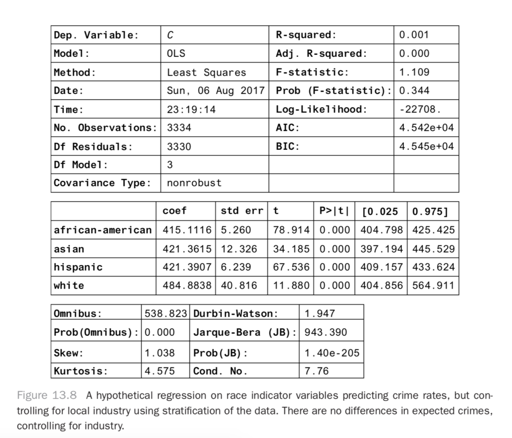
Now you can see that all of the results are within confidence of each other! The dependence between race and crime is fully explained by the industry in the area. In other words, in this hypothetical data set, crime is independent of race when you know what the dominant industry is in the area. What you have done is the same as the conditioning you did before.
Notice that the confidence intervals on the new coefficients are fairly wide compared to what they were before. This is because you’ve restricted to a small subset of your data. Can you do better, maybe by using more of the data? It turns out there’s a better way to control for something than restricting the data set. You can just regress on the variables you’d like to control for!
from statsmodels.api import GLM
import statsmodels.api as sm
races = {0: 'african-american', 1: 'hispanic',
    2: 'asian', 3: 'white'}
X['race'] = X['$R$'].apply(lambda x: races[x])
race_dummies = pd.get_dummies(X['race'])
X[race_dummies.columns] = race_dummies
industries = {i: 'industry_{}'.format(i) for i in range(3)}
    X['industry'] = X['$E$'].apply(lambda x: industries[x])
industry_dummies = pd.get_dummies(X['industry'])
X[industry_dummies.columns] = industry_dummies
x = list(industry_dummies.columns)[1:] + list(race_dummies.columns)
model = OLS(X['$C$'], X[x])
result = model.fit()
result.summary()Then, you get Figure 13.9 shows the result.
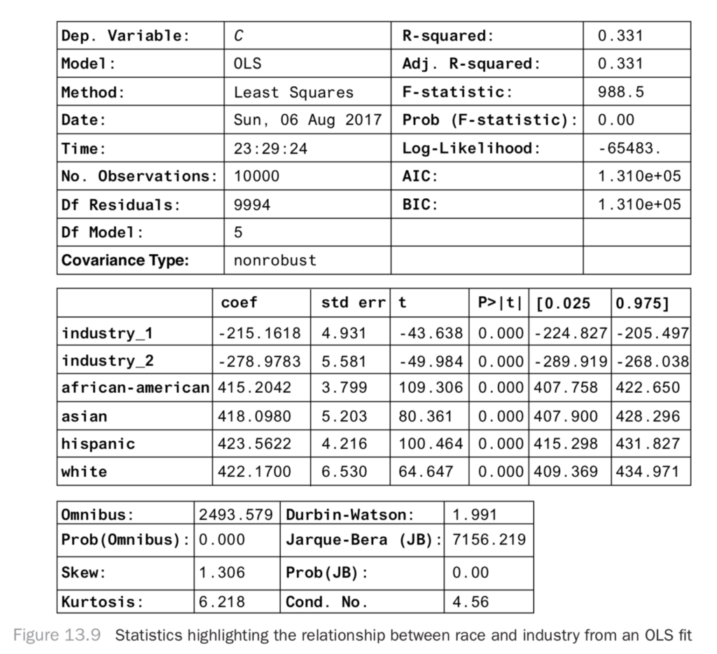
Here, the confidence intervals are much narrower, and you see there’s still no significant association between race and income level: the coefficients are roughly equal. This is a causal regression result: you can now see that there would be no effect of an intervention to change the racial composition of neighborhoods. This simple example is nice because you can see what to control for, and you’ve measured the things you need to control for. How do you know what to control for in general? Will you always be able to do it successfully? It turns out it’s very hard in practice, but sometimes it’s the best you can do.
13.4 Controlling to Block Non-causal Paths
You just saw that you can take a correlative result and make it a causal result by controlling for the right variables. How do you know what variables to control for? How do you know that regression analysis will control for them? This section relies heavily on d-separation from Chapter 11. If that material isn’t fresh, you might want to review it now.
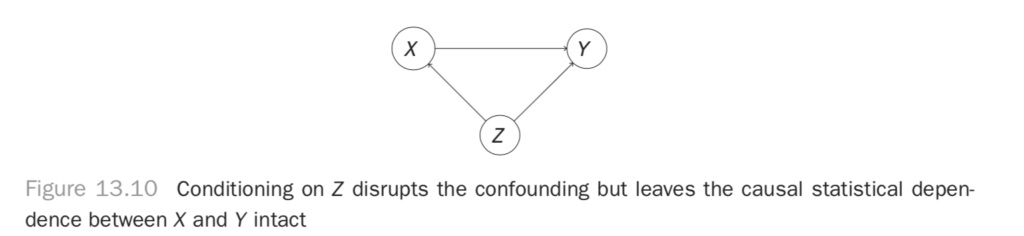
You saw in the previous chapter that conditioning can break statistical dependence. If you condition on the middle variable of a path X → Y → Z, you’ll break the dependence between X and Z that the path produces. If you condition on a confounding variable X ← Z → Y, you can break the dependence between X and Y induced by the confounder as well. It’s important to note that statistical dependence induced by other paths between X and Y is left unharmed by this conditioning. If, for example, you condition on Z in the system in Figure 13.10, you’ll get rid of the confounding but leave the causal dependence.
If you had a general rule to choose which paths to block, you could eliminate all noncausal dependence between variables but save the causal dependence. The “back-door” criterion is the rule you’re looking for. It tells you what set of variables, Z, you should control for to eliminate any noncausal statistical dependence between Xi and Xj. You should note a final nuance before introducing the criterion. If you want to know if the correlation between Xi and Xj is “causal,” you have to worry about the direction of the effect. It’s great to know, for example, that the correlation “being on vacation” and “being relaxed” is not confounded, but you’d really like to know whether “being on vacation” causes you to “be relaxed.” That will inform a policy of going on vacation in order to be relaxed. If the causation were reversed, you couldn’t take that policy.
With that in mind, the back-door criterion is defined relative to an ordered pair of variables, (Xi, Xj), where Xi will be the cause, and Xj will be the effect.
Definition 13.1. Back-Door Conditioning
It’s sufficient to control for a set of variables, Z, to eliminate noncausal dependence for the effect of Xi on Xj in a causal graph, G, if
* No variable in Z is a descendant of Xi, and
* Z blocks every path between Xi and Xj that contains an arrow into Xi.
We won’t prove this theorem, but let’s build some intuition for it. First, let’s examine the condition “no variable in Z is a descendant of Xi.” You learned earlier that if you condition on a common effect of Xi and Xj, then the two variables will be conditionally dependent, even if they’re normally independent. This remains true if you condition on any effect of the common effect (and so on down the paths). Thus, you can see that the first part of the back-door criterion prevents you from introducing extra dependence where there is none.
There is something more to this condition, too. If you have a chain like Xi → Xk → Xj, you see that Xk is a descendant of Xi. It’s not allowed in Z. This is because if you condition on Xk, you’d block a causal path between Xi and Xj. Thus, you see that the first condition also prevents you from conditioning on variables that fall along causal paths.
The second condition says “Z blocks every path between Xi and Xj that contains an arrow into Xi.” This part will tell us to control for confounders. How can you see this? Let’s consider some cases where there is one or more node along the path between Xi and Xj and the path contains an arrow into Xi. If there is a collider along the path between Xi and Xj, then the path is already blocked, so you just condition on the empty set to block that path. Next, if there is a fork along the path, like the path Xi ← Xk → Xj, and no colliders, then you have typical confounding. You can condition on any node along the path that will block it. In this case, you add Xk to the set Z. Note that there can be no causal path from Xi to Xj with an arrow pointing into Xi because of the arrow pointing into Xi.
Thus, you can see that you’re blocking all noncausal paths from Xi to Xj, and the remaining statistical dependence will be showing the causal dependence of Xj on Xi. Is there a way you can use this dependence to estimate the effects of interventions?
13.4.1 The G-formula
Let’s look at what it really means to make an intervention. What it means is that you have a graph like in Figure 13.11.
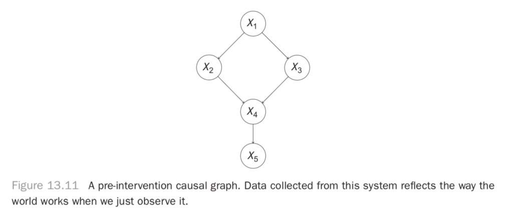
Figure 13.11 A pre-intervention causal graph. Data collected from this system reflects the way the world works when we just observe it.
You want to estimate the effect of X2 on X5. That is, you want to say “If I intervene in this system to set the value of X2 to x2, what will happen to X5? To quantify the effect, you have to realize that all of these variables are taking on values that depend not only on their predecessors but also on noise in the system. Thus, even if there’s a deterministic effect of X2 on X5 (say, raising the value of X5 by exactly one unit), you can only really describe the value X5 will take with a distribution of values. Thus, when you’re estimating the effect of X2 on X5, what you really want is the distribution of X5 when you intervene to set the value of X2.
Let’s look at what we mean by intervene. We’re saying we want to ignore the usual effect of X1 on X2 and set the value of X2 to x2 by applying some external force (our action) to X2. This removes the usual dependence between X2 and X1 and disrupts the downstream effect of X1 on X4 by breaking the path that passes through X2. Thus, we’ll also expect the marginal distribution between X1 and X4, P(X1, X4) to change, as well as the distribution of X1 and X5! Our intervention can affect every variable downstream from it in ways that don’t just depend on the value x2. We actually disrupt other dependences.
You can draw a new graph that represents this intervention. At this point, you’re seeing that the operation is very different from observing the value of X2 = x2, i.e., simply conditioning on X2 = x2. This is because you’re disrupting other dependences in the graph. You’re actually talking about a new system described by the graph in Figure 13.12.
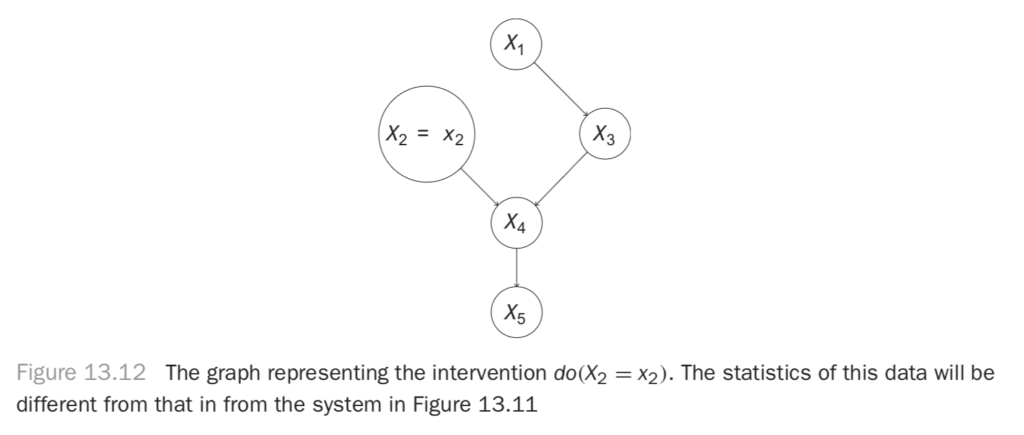
You need some new notation to talk about an intervention like this, so you’ll denote do(X2 = x2) the intervention where you perform this operation. This gives you the definition of the intervention, or do-operation.
Definition 13.2. Do-operation
We describe an intervention called the do() operation in a system described by a DAG, G as an operation where we do Xi by
Delete all edges in G that point into Xi, and
Set the value of Xi to xi.
What does the joint distribution look like for this new graph? Let’s use the usual factorization, and write the following:

Here we’ve just indicated P(X2) by the δ-function, so P(X2) = 0if X2 ≠ x2, and P(X2) = 1 when X2 = x2. We’re basically saying that when we intervene to set X2 = x2, we’re sure that it worked. We can carry through that X2 = x2 elsewhere, like in the distribution for P(X4|X2, X3), but just replacing X2 with X2 = x2, since the whole right-hand side is zero if X2 ̸= x2.
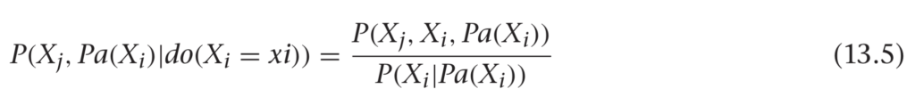
Finally, let’s just condition on the X2 distribution to get rid of the weirdness on the right-hand side of this formula. We can write the following:

To be precise,

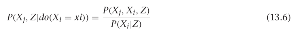
Incredibly, this formula works in general. We can write the following:
This leads us to a nice general rule: the parents of a variable will always satisfy the back-door criterion! It turns out we can be more general than this even. If we marginalize out everything except Xi and Xj, we see the parents are the set of variables that control confounders.
It turns out (we’ll state without proof) that you can generalize the parents to any set, Z, that satisfies the back door criterion.
You can marginalize Z out of this and use the definition of conditional probability to write an important formula, shown in
Definition 13.3.
Definition 13.3. Robins G-Formula
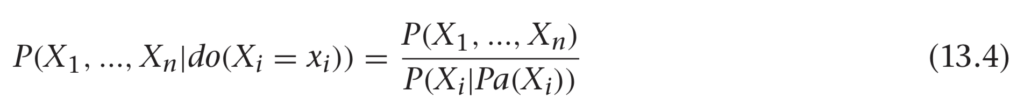
This is a general formula for estimating the distribution of Xj under the intervention Xi. Notice that all of these distributions are from the pre-intervention system. This means you can use observational data to estimate the distribution of Xj under some hypothetical intervention!
There are a few critical caveats here. First, the term in the denominator of Equation 13.4 P(Xi|Pa(Xi)), must be nonzero for the quantity on the left side to be defined. This means you would have to have observed Xi taking on the value you’d like to set it to with your intervention. If you’ve never seen it, you can’t say how the system might behave in response to it!
Next, you’re assuming that you have a set Z that you can control for. Practically, it’s hard to know if you’ve found a good set of variables. There can always be a confounder you have never thought to measure. Likewise, your way of controlling for known confounders might not do a very good job. You’ll understand this second caveat more as you go into some machine learning estimators.
With these caveats, it can be hard to estimate causal effects from observational data. You should consider the results of a conditioning approach to be a provisional estimate of a causal effect. If you’re sure you’re not violating the first condition of the back-door criterion, then you can expect that you’ve removed some spurious dependence. You can’t say for sure that you’ve reduced bias.
Imagine, for example, two sources of bias for the effect of Xi on Xj. Suppose you’re interested in measuring an average value of
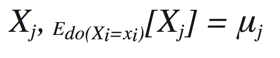
Path A introduces a bias of −δ, and path B introduces a bias of 2δ. If you estimate the mean without controlling for either path, you’ll find
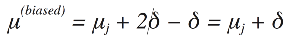
If you control for a confounder along path A, then you remove itsj (biased,A) contribution to the bias, which leaves
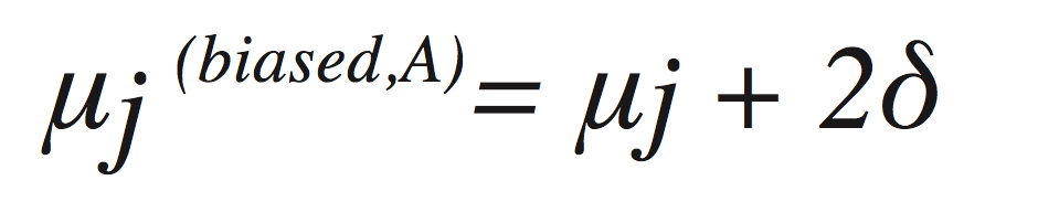
Now the bias is twice as large! The problem, of course, is that the bias you corrected was actually pushing our estimate back toward its correct value. In practice, more controlling usually helps, but you can’t be guaranteed that you won’t find an effect like this. Now that you have a good background in observational causal inference, let’s see how machine-learning estimators can help in practice!
13.5 Machine-Learning Estimators
In general, you won’t want to estimate the full joint distribution under an intervention. You may not even be interested in marginals. Usually, you’re just interested in a difference in average effects.
In the simplest case, you’d like to estimate the expected difference in some outcome, Xj, per unit change in a variable you have control over, Xi. For example, you’d might like to measure
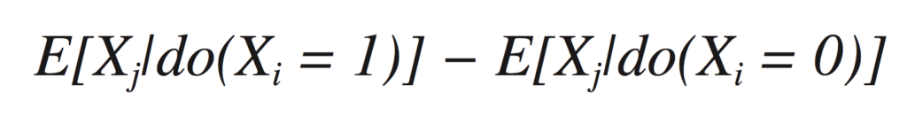
This tells you the change in Xj you can expect on average when you set Xi to 1 from what it would be if Xi were set to 0.
Let’s revisit the g-formula to see how can measure these kinds of quantities.
13.5.1 The G-formula Revisited
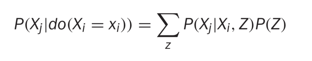
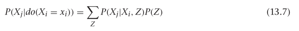
The g-formula tells you how to estimate a causal effect, P(Xj|do(Xi = xi)), using observational data and a set of variables to control for (based on our knowledge of the causal structure). It says this:
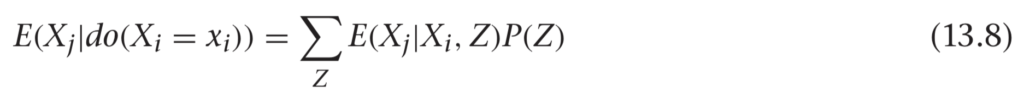
If you take expectation values on each side (by multiplying by Xj and summing over Xj), then you find this:
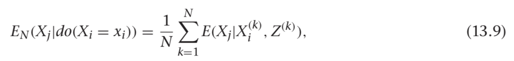
In practice, it’s easy to estimate the first factor on the right side of this formula. If you fit a regression estimator using mean-squared error loss, then the best fit is just the expected value of Xj at each point (Xi, Z). As long as the model has enough freedom to accurately describe the expected value, you can estimate this first factor by using standard machine-learning approaches.
To estimate the whole left side, you need to deal with the P(Z) term, as well as the sum. It turns out there’s a simple trick for doing this. If your data was generated by drawing from the observational joint distribution, then your samples of Z are actually just draws from P(Z). Then, if you replace the P(Z) term by 1/N (for N samples) and sum over data points, you’re left with an estimator for this sum. That is, you can make the substitution as follows:
13.5.2 An Example
Let’s go back to the graph in Figure 13.11. We’ll use an example from Judea Pearl’s book. We’re concerned with the sidewalk being slippery, so we’re investigating its causes. X5 can be 1 or 0, for slippery or not, respectively. You’ve found that the sidewalk is slippery when it’s wet, and you’ll use X4 to indicate whether the sidewalk is wet. Next, you need to know the causes of the sidewalk being wet. You see that a sprinkler is near the sidewalk, and if the sprinkler is on, it makes the sidewalk wet. X2 will indicate whether the sprinkler is on. You’ll notice the sidewalk is also wet after it rains, which you’ll indicate with X3 being 1 after rain, 0 otherwise. Finally, you note that on sunny days you turn the sprinkler on. You’ll indicate the weather with X1, where X1 is 1 if it is sunny, and 0 otherwise.
In this picture, rain and the sprinkler being on are negatively related to each other. This statistical dependence happens because of their mutual dependence on the weather. Let’s simulate some data to explore this system. You’ll use a lot of data, so the random error will be small, and you can focus your attention on the bias.
import numpy as np
import pandas as pd
from scipy.special import expit

N = 100000
inv_logit = expit
x1 = np.random.binomial(1, p=0.5, size=N)
x2 = np.random.binomial(1, p=inv_logit(-3.*x1))
x3 = np.random.binomial(1, p=inv_logit(3.*x1))
x4 = np.bitwise_or(x2, x3)
x5 = np.random.binomial(1, p=inv_logit(3.*x4))
X = pd.DataFrame({'$x_1$': x1, '$x_2$': x2, '$x_3$': x3,
    '$x_4$': x4, '$x_5$': x5})
Every variable here is binary. You use a logistic link function to make logistic regression appropriate. When you don’t know the data-generating process, you might get a little more creative. You’ll come to this point in a moment!
Let’s look at the correlation matrix, shown in Figure 13.13. When the weather is good, the sprinkler is turned on. When it rains, the sprinkler is turned off. You can see there’s a negative relationship between the sprinkler being on and the rain due to this relationship.
There are a few ways you can get an estimate for the effect of X2 on X5. The first is simply by finding the probability that X5 = 1 given that X2 = 1 or X2 = 0. The difference in these probabilities tells you how much more likely it is that the sidewalk is slippery given that the sprinkler was on. A simple way to calculate these probabilities is simply to average the X5 variable in each subset of the data (where X2 = 0 and X2 = 1). You can run the following, which produces the table in Figure 13.14.
X.groupby('$x_2$').mean()[['$x_5$']]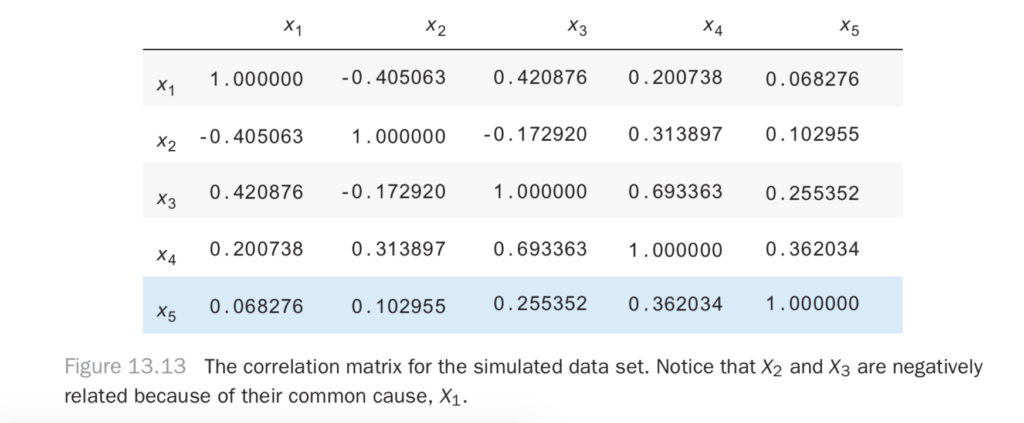
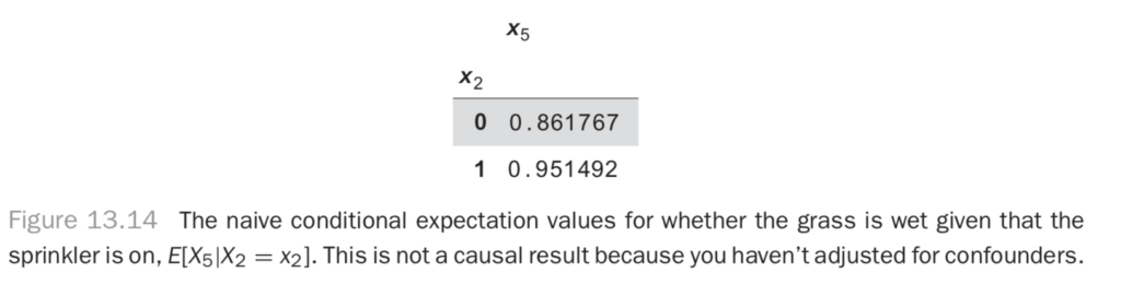
If you look at the difference here, you see that the sidewalk is 0.95 − 0.86 = 0.09, or nine percentage points more likely to be slippery given that the sprinkler was on. You can compare this with the interventional graph to get the true estimate for the change. You can generate this data using the process shown here:
N = 100000
inv_logit = expit
x1 = np.random.binomial(1, p=0.5, size=N)
x2 = np.random.binomial(1, p=inv_logit(-3.*x1))
x3 = np.random.binomial(1, p=inv_logit(3.*x1))
x4 = np.bitwise_or(x2, x3)
x5 = np.random.binomial(1, p=inv_logit(3.*x4))
X = pd.DataFrame({'$x_1$': x1, '$x_2$': x2, '$x_3$': x3,
    '$x_4$': x4, '$x_5$': x5})
Now, X2 is independent of X1 and X3. If you repeat the calculation from before (try it!), you get a difference of 0.12, or 12 percentage points. This is about 30 percent larger than the naive estimate!
Now, you’ll use some machine learning approaches to try to get a better estimate of the true (0.12) effect strictly using the observational data. First, you’ll try a logistic regression on the first data set. Let’s re-create the naive estimate, just to make sure it’s working properly.
from sklearn.linear_model import LogisticRegression
# build our model, predicting $x_5$ using $x_2$
model = LogisticRegression()
model = model.fit(X[['$x_2$']], X['$x_5$'])

# what would have happened if $x_2$ was always 0:
X0 = X.copy()
X0['$x_2$'] = 0
y_pred_0 = model.predict_proba(X0[['$x_2$']])

# what would have happened if $x_2$ was always 1:
X1 = X.copy()
X1['$x_2$'] = 1
y_pred_1 = model.predict_proba(X1[['$x_2$']])
# now, let's check the difference in probabilities
y_pred_1[:, 1].mean() - y_pred_0[:,1].mean()
You first build a logistic regression model using X2 to predict X5. You do the prediction and use it to get probabilities of X5 under the X2 = 0 and X2 = 1 states. You did this over the whole data set.
The reason for this is that you’ll often have more interesting data sets, with many more variables changing, and you’ll want to see the average effect of X2 on X5 over the whole data set. This procedure lets you do that. Finally, you find the average difference in probabilities between the two states, and you get the same 0.09 result as before!
Now, you’d like to do controlling on the same observational data to get the causal (0.12) result. You perform the same procedure as before, but this time you include X1 in the regression.
model = LogisticRegression()
model = model.fit(X[['$x_2$', '$x_1$']], X['$x_5$'])# what would have happened if $x_2$ was always 0:
X0 = X.copy()
X0['$x_2$'] = 0
y_pred_0 = model.predict_proba(X0[['$x_2$', '$x_1$']])

# what would have happened if $x_2$ was always 1:
X1 = X.copy()
X1['$x_2$'] = 1

# now, let's check the difference in probabilities
y_pred_1 = model.predict_proba(X1[['$x_2$', '$x_1$']])
y_pred_1[:, 1].mean() - y_pred_0[:,1].mean()
In this case, you find 0.14 for the result. You’ve over-estimated it! What went wrong? You didn’t actually do anything wrong with the modeling procedure. The problem is simply that logistic regression isn’t the right model for this situation. It’s the correct model for each variable’s parents to predict its value but doesn’t work properly for descendants that follow the parents. Can we do better, with a more general model?
This will be your first look at how powerful neural networks can be for general machine-learning tasks. You’ll learn about building them in a little more detail in the next chapter. For now, let’s try a deep feedforward neural network using keras. It’s called deep because there are more than just the input and output layers. It’s a feedforward network because you put some input data into the network and pass them forward through the layers to produce the output.
Deep feedforward networks have the property of being “universal function approximators,” in the sense that they can approximate any function, given enough neurons and layers (although it’s not always easy to learn, in practice). You’ll construct the network like this:
from keras.layers import Dense, Input
from keras.models import Model
dense_size = 128
input_features = 2
x_in = Input(shape=(input_features,))
h1 = Dense(dense_size, activation='relu')(x_in)
h2 = Dense(dense_size, activation='relu')(h1)
h3 = Dense(dense_size, activation='relu')(h2)
y_out = Dense(1, activation='sigmoid')(h3)

model = Model(input=x_in, output=y_out)
model.compile(loss='binary_crossentropy', optimizer='adam')
model.fit(X[['$x_1$', '$x_2$']].values, X['$x_5$'])
Now do the same prediction procedure as before, which produces the result 0.129.
X_zero = X.copy()
X_zero['$x_2$'] = 0
x5_pred_0 = model.predict(X_zero[['$x_1$', '$x_2$']].values)
X_one = X.copy()
X_one['$x_2$'] = 1
x5_pred_1 = model.predict(X_one[['$x_1$', '$x_2$']].values)
x5_pred_1.mean() - x5_pred_0.mean()
You’ve done better than the logistic regression model! This was a tricky case. You’re given binary data where it’s easy to calculate probabilities, and you’d do the best by simply using the g-formula directly. When you do this (try it yourself!), you calculate the true result of 0.127 from this data. Your neural network model is very close!
Now, you’d like to enact a policy that would make the sidewalk less likely to be slippery. You know that if you turn the sprinkler on less often, that should do the trick. You see that enacting this policy (and so intervening to change the system), you can expect the slipperiness of the sidewalk to decrease. How much? You want to compare the pre-intervention chance of slipperiness with the post-intervention chance, when you set sprinkler = off. You can simply calculate this with our neural network model like so:
X['$x_5$'].mean() - x5_pred_0.mean()This gives the result 0.07. It will be 7 percent less likely that the sidewalk is slippery if you make a policy of keeping the sprinkler turned off!
13.6 Conclusion
In this chapter, you’ve developed the tools to do causal inference. You’ve learned that machine learning models can be useful to get more general model specifications, and you saw that the better you can predict an outcome using a machine learning model, the better you can remove bias from an observational causal effect estimate.
Observational causal effect estimates should always be used with care. Whenever possible, you should try to do a randomized controlled experiment instead of using the observational estimate. In this example, you should simply use randomized control: flip a coin each day to see whether the sprinkler gets turned on. This re-creates the post-intervention system and lets you measure how much less likely the sidewalk is to be slippery when the sprinkler is turned off versus turned on (or when the system isn’t intervened upon). When you’re trying to estimate the effect of a policy, it’s hard to find a substitute for actually testing the policy through a controlled experiment.
It’s especially useful to be able to think causally when designing machine-learning systems. If you’d simply like to say what outcome is most likely given what normally happens in a system, a standard machine learning algorithm is appropriate. You’re not trying to predict the result of an intervention, and you’re not trying to make a system that is robust to changes in how the system operates. You just want to describe the system’s joint distribution (or expectation values under it).
If you would like to inform policy changes, predict the outcomes of intervention, or make the system robust to changes in variables upstream from it (i.e., external interventions), then you will want a causal machine learning system, where you control for the appropriate variables to measure causal effects.
An especially interesting application area is when you’re estimating the coefficients in a logistic regression. Earlier, you saw that logistic regression coefficients had a particular interpretation in observational data: they describe how much more likely an outcome is per unit increase in some independent variable. If you control for the right variables to get a causal logistic regression estimate (or just do the regression on data generated by control), then you have a new, stronger interpretation: the coefficients tell you how much more likely an outcome is to occur when you intervene to increase the value of an independent variable by one unit. You can use these coefficients to inform policy!

Domino powers model-driven businesses with its leading Enterprise AI platform that accelerates the development and deployment of data science work while increasing collaboration and governance. More than 20 percent of the Fortune 100 count on Domino to help scale data science, turning it into a competitive advantage. Founded in 2013, Domino is backed by Sequoia Capital and other leading investors.
Other posts you might be interested in


Subscribe to the Domino Newsletter
Receive data science tips and tutorials from leading Data Science leaders, right to your inbox.
By submitting this form you agree to receive communications from Domino related to products and services in accordance with Domino's privacy policy and may opt-out at anytime.